Probability and likelihood distributions

The probability of a value can mean its probability of being the true value of some parameter θ, conditional on some model M or ensemble of models. It can also mean the probability of observing that value, again conditional on some model M or ensemble of models. Either way we can express it as P(θ|M).

For discrete parameters these probabilities are probability masses. The masses for all possible values of the parameter, which are finite in number, must sum to be 1 because one of those values of that parameter must be correct or be observed (conditional on some model).

Put another way, we cannot have missing probability, which implies that the range of values being considered is incomplete. We also cannot have excess probability, which implies that multiple values could be true at the same time.

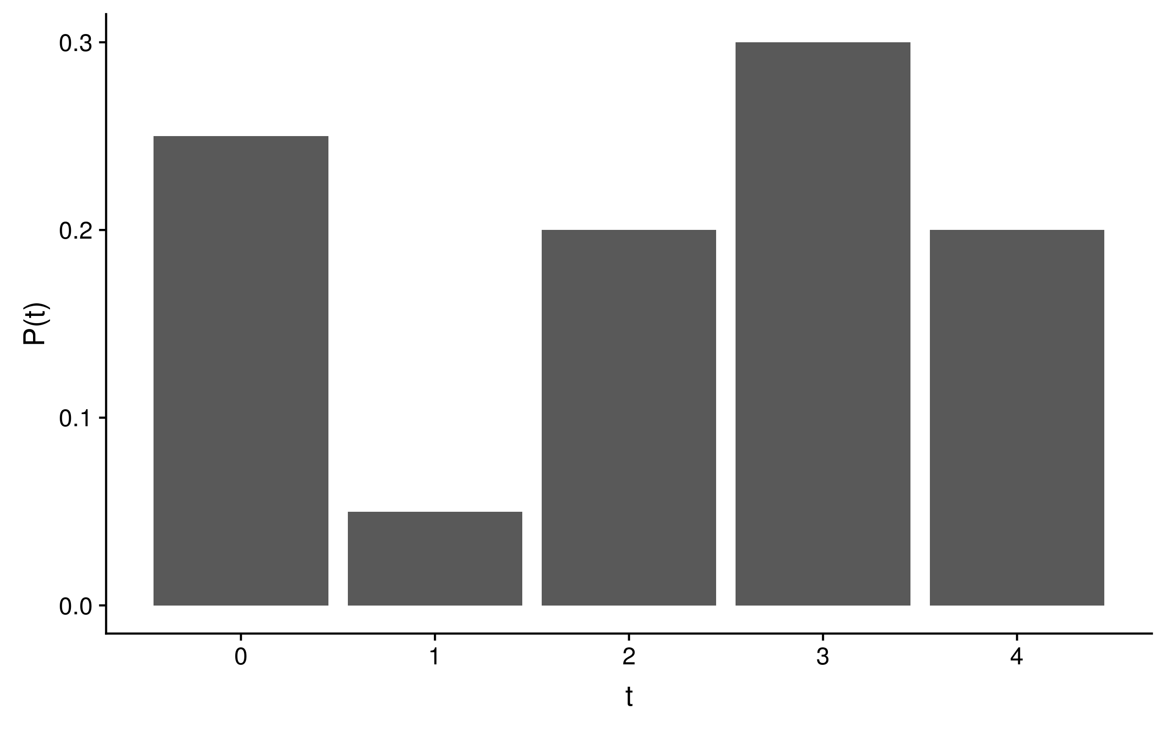
Consider a probability distribution for some time parameter t, with five discrete time steps from 0 to 4. This distribution has only four free parameters because whatever the probabilities of time steps 0 through 3 are, the value of time step 4 must be 1 minus the sum of P(t = 0) through P(t = 3). The following probability mass distribution is valid because the five probabilities (0.25, 0.05, 0.2, 0.3 and 0.2) sum to 1:

For continuous parameters, the probabilities are probability densities. There are infinite possible values for a continuous parameter, and the distribution must integrate to 1.

Consider a probability distribution for some time parameter t with a lower bound of 0 which decays linearly from time t = 0, until the probability P(t = 4) = 0. This will be a right angled triangle which has an area of (a × b) / 2, where a and b are the lengths of the opposite and adjacent sides.

Since the integral over P(t) dt must equal 1 for this distribution to be a genuine probability distribution, (a × b) / 2 = 1. Since b = 4, P(t) = a = 2 / b = 2 / 4 = 0.5. The probability distribution will look like this:

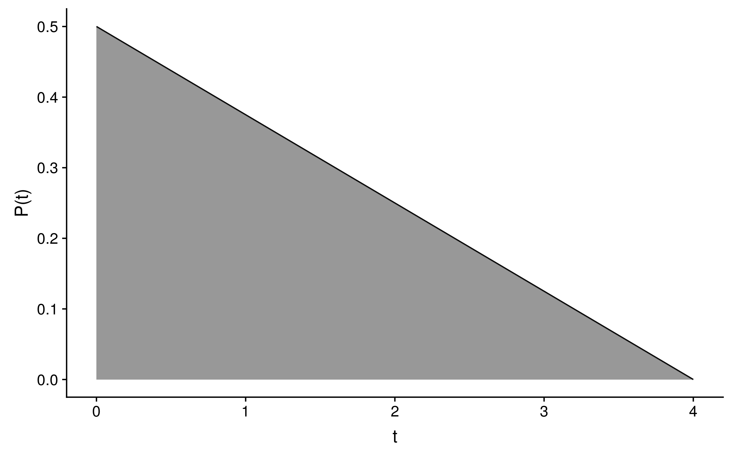
This probability distribution has one free parameter, because the value of a will determine the value of b and vice versa.

The likelihood of θ is the probability of observing data D, given a model M and θ of parameter values - P(D|M,θ). A likelihood distribution will not sum to one, because there is no reason for the sum or integral of likelihoods over all parameter values to sum to one.

Consider a model where the data is some observed temperature, the model is a grid of the Earth’s surface, and the model parameter value is the grid cell (or pixel) that temperature was observed in. The likelihood is the probability of observing that temperature (the data) given it was observed in a particular grid cell (the parameter value).

If the observed temperature T was say minus 100 celsius, the probability of observing it would be extremely low for all grid cells, even those in Antarctica. So the sum of likelihoods over all grid cells will be less than 1.

The sum or integral over all likelihoods can even be greater than 1! Imagine that the following probability distribution is the distribution of temperatures for one grid cell:

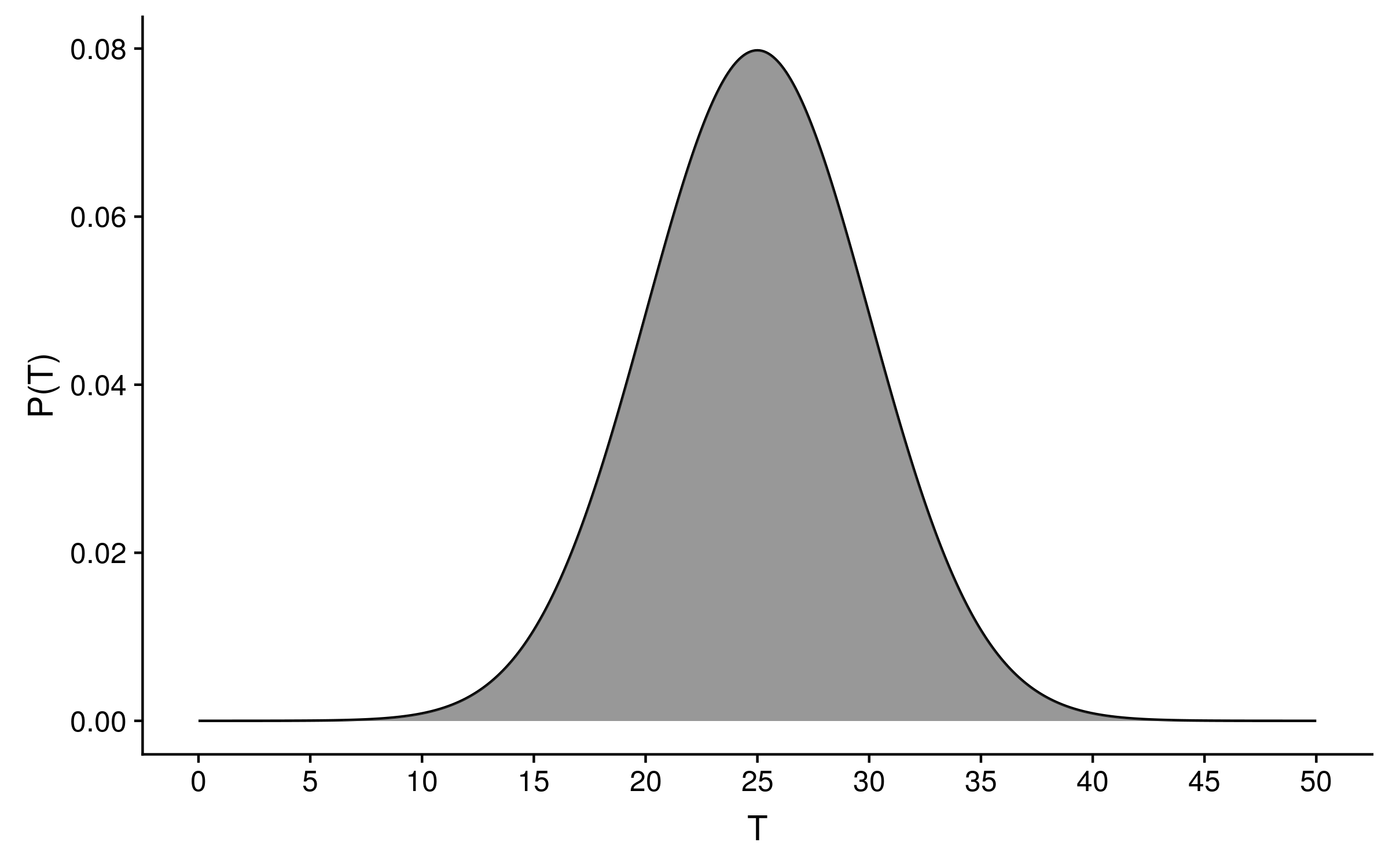
This is a genuine probability distribution, because the area under the curve sums to 1. Now imagine 1000 grid cells each have the same temperature distribution as above. If our observed temperature data point T = 25 degrees celsius, the sum of likelihoods across those 1000 grid cells will be 0.08 × 1000 = 80! Clearly likelihood distributions are not genuine probability distributions, otherwise we could have an 8,000% probability of observing the data!