<?xml version="1.0" encoding="utf-8"?><feed xmlns="http://www.w3.org/2005/Atom" ><generator uri="https://jekyllrb.com/" version="4.3.1">Jekyll</generator><link href="https://cs.rice.edu/~ogilvie/feed.xml" rel="self" type="application/atom+xml" /><link href="https://cs.rice.edu/~ogilvie/" rel="alternate" type="text/html" /><updated>2022-10-26T19:44:49-05:00</updated><id>https://cs.rice.edu/~ogilvie/feed.xml</id><title type="html">Species and Gene Evolution</title><subtitle>Where I share information about my research and teaching.</subtitle><author><name>Huw A. Ogilvie</name></author><entry><title type="html">PAM (Dayhoff) matrices</title><link href="https://cs.rice.edu/~ogilvie/comp571/pam/" rel="alternate" type="text/html" title="PAM (Dayhoff) matrices" /><published>2022-10-06T09:00:00-05:00</published><updated>2022-10-06T09:00:00-05:00</updated><id>https://cs.rice.edu/~ogilvie/comp571/pam</id><content type="html" xml:base="https://cs.rice.edu/~ogilvie/comp571/pam/"><![CDATA[<p>The point accepted mutation (PAM) substitution model, also known as the Dayhoff substitution model, is an amino acid substitution model derived from empirical observation of mutations among closely related proteins. This venerable model was described in various volumes and supplements of the <em>Atlas of Protein Sequence and Structure</em>, with the most well-known version being published in the 1978 supplement by Dayhoff, Schwartz and Orcutt.</p>

<p>Since 1966, Dayhoff and her colleagues had been collecting and compiling protein sequences into their <em>Atlas</em>, and groups of closely related sequences from the <em>Atlas</em> were used as the basis for the PAM matrix. Where more than two sequences were in a group, phylogenetic trees were inferred along with ancestral sequences on each node of the tree, presumably using a method similar to the one published by Eck and Dayhoff in 1966. This method has been variously described as maximum parsimony (e.g. in <a href="https://doi.org/10.1007/PL00000067">Zhang and Nei 1996</a>) or minimum evolution (e.g. in <a href="https://doi.org/10.1093/sysbio/45.1.79">Edwards 1996</a>).</p>

<p>Maximum parsimony (MP) methods optimize for the smallest possible number of mutations; for a given tree there will be a minimum number of mutations required to explain the known sequences, and MP methods attempt to find the tree with the smallest minimum number of mutations.</p>

<p>Each branch of a tree is associated with a pair of sequences, one at either end of the branch. These pairs of sequences were extracted from each tree. For each pair of sequences either from a tree or from the groups of size two, if there were two different amino acids at a given position it was assumed that a single mutation - a PAM - had occured, directly changing the amino acid of one of the sequences to the amino acid of the other sequence. This assumption is justified on the basis that sequences will be closely related enough that only one or zero mutations are likely to have occured at each site within these pairs. Models of sequence evolution making this assumption are commonly known as infinite-sites models (e.g. in <a href="https://doi.org/10.1093/genetics/143.3.1457">Tajima 1996</a>). If this assumption holds, then the vector of <strong>counts</strong> of mutations from one amino acid to the other nineteen amino acids should be proportional to the <strong>rates</strong> of transition from that one amino acid to the other nineteen, albeit with some sampling error.</p>

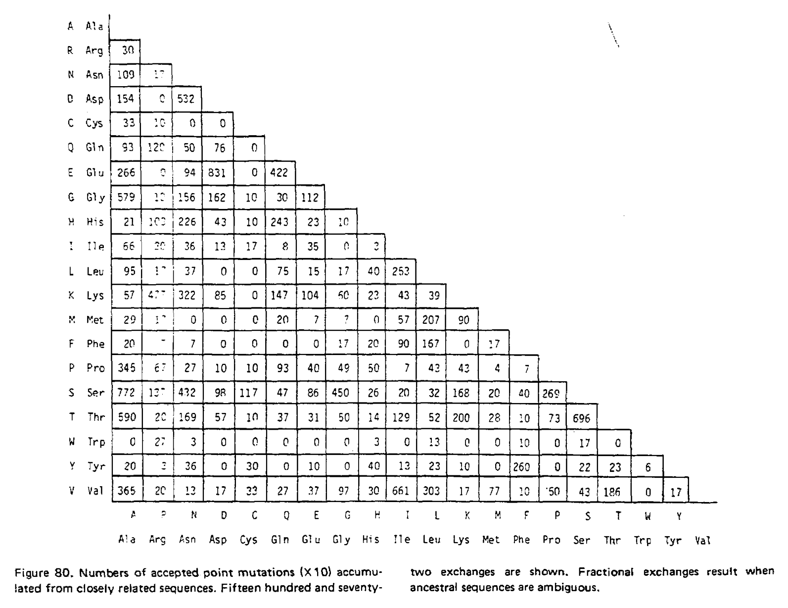
<p>In the 1978 version of the matrix, 71 groups were identified containing 1,572 mutations in total. Using the above procedure, point accepted mutations occuring in this dataset were counted and recorded in a matrix called A. This is a triangular matrix because the process is assumed to be reversible conditional on there being a mutation from the initial state; the probability of a mutation from state X to state Y, conditional on there being a mutation from state X to anything else, is the same as a mutation from Y to X conditional on there being a mutation from Y to anything else. Here is the count matrix:</p>

<p><img src="https://cs.rice.edu/~ogilvie/assets/pam_count_matrix.png" alt="PAM count matrix M" /></p>

<p>We want to transform this matrix into a transition probability matrix M. Given some alphabet of states C, that matrix gives us the probability of a particular end state C<sub><em>i</em></sub> (in this case, a particular amino acid) given an initial state C<sub><em>j</em></sub> and some duration of time <em>t</em>, which we can write as M<sub><em>ij</em></sub> = P(C<sub><em>i</em></sub>|C<sub><em>j</em></sub>, <em>t</em>). For the case where a mutation has definitely occured and <em>i</em> is different from <em>j</em>, we can express this as the joint probability P(C<sub><em>i</em></sub>, <em>i</em> ≠ <em>j</em>|C<sub><em>j</em></sub>, <em>t</em>), which will correspond to the off-diagonal elements of M. Following the chain rule, we can decompose this joint probability into P(C<sub><em>i</em></sub>|C<sub><em>j</em></sub>, <em>i</em> ≠ <em>j</em>, <em>t</em>)P(<em>i</em> ≠ <em>j</em>|C<sub><em>j</em></sub>, <em>t</em>). When <em>t</em> is small enough that the infinite sites assumption is reasonable, then the probability of C<sub><em>i</em></sub> conditioned on <em>i</em> ≠ <em>j</em> will not depend on <em>t</em>, and this formulation can be approximated as P(C<sub><em>i</em></sub>|C<sub><em>j</em></sub>, <em>i</em> ≠ <em>j</em>)P(<em>i</em> ≠ <em>j</em>|C<sub><em>j</em></sub>, <em>t</em>).</p>

<p>We can estimate P(C<sub><em>i</em></sub>|C<sub><em>j</em></sub>, <em>i</em> ≠ <em>j</em>) from the symmetric version of the above triangular matrix of counts, by transforming the count of <em>j</em> to <em>i</em> mutations A<sub><em>ij</em></sub> into a proportion by dividing this count by the total number of all mutations starting with <em>j</em>, or Σ<sub><em>i</em></sub>A<sub><em>ij</em></sub>. To compute the probability of any mutation P(<em>i</em> ≠ <em>j</em>|C<sub><em>j</em></sub>, <em>t</em>), first the relative “mutability” m of each amino acid was calculated, a value which is proportional to (but not equal to) that probability when <em>t</em> is small enough that multiple mutations are unlikely. Put another way, m<sub><em>j</em></sub> is approximately proportional to P(<em>i</em> ≠ <em>j</em>|C<sub><em>j</em></sub>, <em>t</em>) for any small value of <em>t</em>. To derive the PAM/Dayhoff matrix, mutability was estimated as the number of mutations involving C<sub><em>j</em></sub> relative to the overall occurance of C<sub><em>j</em></sub> across all sequences. This mutability score was normalized so that the mutability of alanine equaled 100, an arbitrary choice given m is only proportional to the desired probabilities.</p>

<p>Finally, for each amino acid, an overall scaling factor λ was used to scale m<sub><em>j</em></sub> from a relative value to the probability of mutation given 1 unit of time, i.e. λm<sub><em>j</em></sub> = P(<em>i</em> ≠ <em>j</em>|C<sub><em>j</em></sub>, <em>t</em> = 1). We can now calculate the off-diagonal values (where i ≠ <em>j</em>) of the transition probability matrix for <em>t</em> = 1 as:</p>

<p><img src="https://cs.rice.edu/~ogilvie/assets/pam_off_diagonal_transition_probability.png" alt="PAM off-diagonal transition probability equation" /></p>

<p>This scaling factor was calculated to set the unconditional mutation probability, that is P(<em>i</em> ≠ <em>j</em>), to equal 0.01 mutations per site, or equivalently equal 1 mutation for every 100 sites, given the resulting substitution matrix and an underlying amino acid frequency distribution. As a result, 1 unit of time is equal to the amount of time in which we expect 0.01 mutations to occur per site, which is called 1 PAM unit. Since whether or not a mutation has occured is a binary choice, the diagonal matrix values for 1 PAM unit, which correspond to P(<em>i</em> = <em>j</em>|C<sub><em>j</em></sub>, <em>t</em> = 1), are equal to 1 - P(<em>i</em> ≠ <em>j</em>|C<sub><em>j</em></sub>, <em>t</em> = 1) or:</p>

<p><img src="https://cs.rice.edu/~ogilvie/assets/pam_diagonal_transition_probability.png" alt="PAM diagonal transition probability equation" /></p>

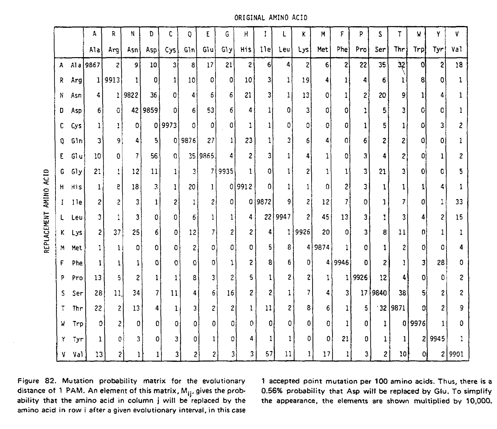
<p>Using these two formulae, Dayhoff and colleagues calculated the entire transition probability matrix for 1 PAM unit:</p>

<p><img src="https://cs.rice.edu/~ogilvie/assets/pam1_transition_probability_matrix.png" alt="PAM1 transition probabilities" /></p>

<p>However, it is unlikely we are analyzing sequences exactly 1 PAM unit apart. As such we need to derive matrices for greater values of <em>t</em>, and in their 1978 supplement Dayhoff and colleagues derived the PAM250 matrix. This was done using matrix multiplication because at larger distances, multiple substitutions become much more likely. To illustrate the use of matrix multiplication to derive PAM<em>n</em> matrices, let’s consider a toy example with just three states; red, green and blue. Here is our transition probability matrix for one time unit:</p>

<table>
  <tbody>
    <tr>
      <td> </td>
      <td>red</td>
      <td>green</td>
      <td>blue</td>
    </tr>
    <tr>
      <td>red</td>
      <td>0.95</td>
      <td>0.08</td>
      <td>0.01</td>
    </tr>
    <tr>
      <td>green</td>
      <td>0.04</td>
      <td>0.84</td>
      <td>0.04</td>
    </tr>
    <tr>
      <td>blue</td>
      <td>0.01</td>
      <td>0.08</td>
      <td>0.95</td>
    </tr>
  </tbody>
</table>

<p>While modern phylogenetic methods treat evolution as a continuous-time Markov chain (CTMC) where each time step is infinitesimally small, in this case I will approximate evolution as a discrete-time Markov chain (DTMC) with time steps of 1 time unit as it is easier to explain.</p>

<p>After one time step, there is only one way a state can remain unchanged; no mutation must have occured. But after two time steps there is another possibility; a mutation occured at the first time step, and was reversed in the second.</p>

<p>For example, if the state is red at the start and end of the process, it could have remained unchanged over two time steps, but could also have mutated to green in the first time step and back to red, or to blue and back. We therefore need to sum over these possibilities to get the probability of remaining red over two time units. We calculate this sum as M<sub>11</sub>×M<sub>11</sub> + M<sub>12</sub>×M<sub>21</sub> + M<sub>13</sub>×M<sub>31</sub> = 0.95×0.95 + 0.04×0.08 + 0.01×0.01 = 0.9058. The same logic applies to every other entry in our matrix, and we can use it to create a the transition probability matrix for two time units:</p>

<table>
  <tbody>
    <tr>
      <td> </td>
      <td>red</td>
      <td>green</td>
      <td>blue</td>
    </tr>
    <tr>
      <td>red</td>
      <td>0.9058</td>
      <td>0.1440</td>
      <td>0.0222</td>
    </tr>
    <tr>
      <td>green</td>
      <td>0.0720</td>
      <td>0.7120</td>
      <td>0.0720</td>
    </tr>
    <tr>
      <td>blue</td>
      <td>0.0222</td>
      <td>0.1440</td>
      <td>0.9058</td>
    </tr>
  </tbody>
</table>

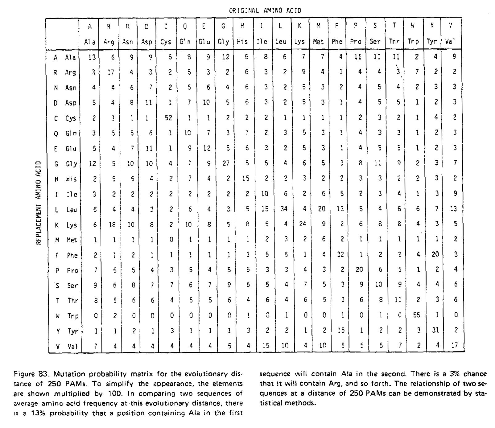
<p>We have just performed <a href="https://en.wikipedia.org/wiki/Matrix_multiplication">matrix multiplication</a>, calculating M×M=M<sup>2</sup>! We could multiply the resulting matrix by M again to get M<sup>3</sup>, the transition probability matrix for three time units. The PAM<em>n</em> matrices were calculated this way, for example the PAM250 matrix:</p>

<p><img src="https://cs.rice.edu/~ogilvie/assets/pam250_transition_probability_matrix.png" alt="PAM250 transition probabilities" /></p>

<p>Notice how the transition probabilities get “flatter” the more time has passed. Given an infinite amount of time, each column would have an identical set of probabilities; the final amino acid would be completely independent of the initial amino acid, and the log-odds scores calculated from these transition probabilities would be identical to the non-homologous log-odds scores.</p>]]></content><author><name>Huw A. Ogilvie</name></author><category term="comp571" /><summary type="html"><![CDATA[The point accepted mutation (PAM) substitution model, also known as the Dayhoff substitution model, is an amino acid substitution model derived from empirical observation of mutations among closely related proteins. This venerable model was described in various volumes and supplements of the Atlas of Protein Sequence and Structure, with the most well-known version being published in the 1978 supplement by Dayhoff, Schwartz and Orcutt.]]></summary></entry><entry><title type="html">COMP571 (Fall 2022)</title><link href="https://cs.rice.edu/~ogilvie/comp571/comp571-fall-2022/" rel="alternate" type="text/html" title="COMP571 (Fall 2022)" /><published>2022-08-22T09:00:00-05:00</published><updated>2022-08-22T09:00:00-05:00</updated><id>https://cs.rice.edu/~ogilvie/comp571/comp571-fall-2022</id><content type="html" xml:base="https://cs.rice.edu/~ogilvie/comp571/comp571-fall-2022/"><![CDATA[<p><strong>Important note:</strong> The information contained in the course syllabus, other than
the absence policies, may be subject to change with reasonable advance notice,
as deemed appropriate by the instructor.</p>

<h1 id="who">Who</h1>

<p>Instructor:</p>

<ul>
  <li>Huw A. Ogilvie</li>
  <li><a href="mailto:hao3@rice.edu">hao3@rice.edu</a></li>
</ul>

<p>TAs:</p>

<ul>
  <li>Jared Slone</li>
  <li><a href="mailto:js201@rice.edu">js201@rice.edu</a></li>
</ul>

<h1 id="where-and-when">Where and when</h1>

<p>Lectures will be held in Maxfield Hall <strong>252</strong>, on Mondays and Wednesdays,
between 4:00–5:15 PM. All lectures will be delivered in-person and, without a
reasonable excuse, attendence is expected. One scheduled office hour will be
held on Zoom, at a time to be determined based on scheduling conflicts, and
attendance by the whole class is encouraged so that everyone can benefit from
the discussion. Office hours will not be recorded. Individual appointments
outside this time are welcome.</p>

<p>Distribution of class materials and submission of assignments and projects
will be conducted via <a href="https://canvas.rice.edu/">Canvas</a>. Slack will be used
for coordination and communication around group projects.</p>

<h1 id="intended-audience">Intended audience</h1>

<p>The students who should take COMP571 are generally studying computer science,
biology or genomics, and wish to learn how to apply algorithms and statistical
models to important problems in biology and genomics.</p>

<h1 id="course-objectives-and-learning-outcomes">Course objectives and learning outcomes</h1>

<p>The primary objective of the course is to teach the theory behind methods in
biological sequence analysis, including sequence alignment, sequence motifs,
and phylogenetic tree reconstruction. By the end of the course, students are
expected to understand and be able to write basic implementations of the
algorithms which power those methods.</p>

<h1 id="course-materials">Course materials</h1>

<p>The main material for this course will be lectures and the course blog. That
said, <em>Statistics for Biology and Health</em> by Ewens &amp; Grant is a good resource
and a PDF copy should be accessible
<a href="https://link.springer.com/book/10.1007/b137845">here</a> or through the Fondren
Library.</p>

<h1 id="software-for-the-course">Software for the course</h1>

<p>Algorithms and statistics will be demonstrated using Python. Assignments and
projects will require some Python coding. R may be used for some
demonstrations (because it is nice for data visualization) but not for
assessment.</p>

<p>The <a href="http://www.numpy.org/">NumPy</a> and <a href="https://www.scipy.org/">SciPy</a>
libraries for scientific computing will be used with Python. To install these
libraries, first install the latest official distribution of Python 3. This
can be downloaded for <a href="https://www.python.org/downloads/mac-osx/">macOS</a> or
for <a href="https://www.python.org/downloads/windows/">Windows</a> from Python.org, and
should already be included with your operating system if you are using Linux.</p>

<p>Then simply use the Python package manage pip to install NumPy and SciPy from
the command line, by running <code class="language-plaintext highlighter-rouge">pip3 install numpy scipy</code>.</p>

<h1 id="schedule-and-assessment">Schedule and assessment</h1>

<p>The course is organized around five themes<del>, and there will be a corresponding
theory-based homework assignment for each one</del>;</p>

<ol>
  <li>Substitution models for gapless alignments</li>
  <li>Global alignment, local alignment, and BLAST</li>
  <li>Hidden Markov Models and transmembrane domain identification</li>
  <li>Sankoff’s and hill climbing algorithms</li>
  <li>Phylogenetic likelihood and coalescent theory</li>
</ol>

<p>Assignments should be completed individually, copying answers without
attribution from other sources including other students will be considered
plagiarism.</p>

<p>In addition to these assignments, each student will have to complete one
project of implementing a novel or existing statistical model, applying it to
a public data set, and writing up the results in the style of a scientific
paper. The statistical model should be relevant to one (or more) of the
course themes. Projects will be designed by groups of 3–5 students, but the
implementation, application and write up will be individual. Copying and
pasting code or your report (in part or in whole) without attribution from
other sources including other students will be considered plagiarism. Project
code and reports will be due on <strong>December 2nd.</strong> A design document will be
due on <strong>November 4th</strong> before the project due date which will be completed
and submitted by the group rather than individually.</p>

<p><em>The below schedule may change subject to Rice University policy</em></p>

<table>
  <thead>
    <tr>
      <th>Monday’s date</th>
      <th>Monday’s lecture</th>
      <th>Wednesday’s lecture</th>
      <th>Homework</th>
    </tr>
  </thead>
  <tbody>
    <tr>
      <td>08/22/22</td>
      <td>Introduction</td>
      <td>Central dogma and gene models</td>
      <td> </td>
    </tr>
    <tr>
      <td>08/29/22</td>
      <td><em>canceled</em></td>
      <td><em>canceled</em></td>
      <td> </td>
    </tr>
    <tr>
      <td>09/05/22</td>
      <td><em>Labor Day, no scheduled classes</em></td>
      <td>Margaret Dayhoff’s <em>Atlas</em><sup>1</sup></td>
      <td> </td>
    </tr>
    <tr>
      <td>09/12/22</td>
      <td>Homology testing using log-odds<sup>2</sup></td>
      <td>Global alignment<sup>2</sup></td>
      <td> </td>
    </tr>
    <tr>
      <td>09/19/22</td>
      <td>Local alignment<sup>2</sup></td>
      <td>BLAST (gapless phase)<sup>2</sup></td>
      <td> </td>
    </tr>
    <tr>
      <td>09/26/22</td>
      <td>BLAST (gapped phase)<sup>2</sup></td>
      <td>Hidden Markov models<sup>3</sup></td>
      <td>#1 issued</td>
    </tr>
    <tr>
      <td>10/03/22</td>
      <td>Viterbi algorithm<sup>3</sup></td>
      <td>Forward algorithm<sup>3</sup></td>
      <td>#1 due</td>
    </tr>
    <tr>
      <td>10/10/22</td>
      <td><em>Midterm recess, no scheduled classes</em></td>
      <td>Backward algorithm<sup>3</sup></td>
      <td> </td>
    </tr>
    <tr>
      <td>10/17/22</td>
      <td><em>canceled</em></td>
      <td>Baum-Welch algorithm</td>
      <td> </td>
    </tr>
    <tr>
      <td>10/24/22</td>
      <td>Phylogenetic trees<sup>4</sup></td>
      <td>Hill climbing<sup>4</sup></td>
      <td>#2 issued</td>
    </tr>
    <tr>
      <td>10/31/22</td>
      <td>The Felsenstein zone<sup>4</sup></td>
      <td>Time-reversible models of evolution<sup>5</sup></td>
      <td>#2 due</td>
    </tr>
    <tr>
      <td>11/07/22</td>
      <td>Felsenstein’s pruning algorithm<sup>5</sup></td>
      <td>Wright–Fisher model<sup>5</sup></td>
      <td> </td>
    </tr>
    <tr>
      <td>11/14/22</td>
      <td>Kingman’s coalescent<sup>5</sup></td>
      <td>Bayesian phylogenetic inference</td>
      <td> </td>
    </tr>
    <tr>
      <td>11/21/22</td>
      <td>Metropolis algorithm</td>
      <td><em>Thanksgiving recess, no scheduled classes</em></td>
      <td>#3 issued</td>
    </tr>
    <tr>
      <td>11/28/22</td>
      <td><em>Buffer</em></td>
      <td><em>Buffer</em></td>
      <td>#3 due</td>
    </tr>
    <tr>
      <td>12/05/22</td>
      <td><em>Scheduled classes finished</em></td>
      <td><em>Scheduled classes finished</em></td>
      <td> </td>
    </tr>
  </tbody>
</table>

<p>Each row in the above table lists the lecture topics, homework and project
milestones for the week beginning on the specified Monday and ending the
following Sunday. Superscript numbers refer to the theme(s) for that day’s
class or midterm. Assignments will be issued before midnight on the <strong>Monday at
the start of the week</strong>. Assignments will also be due before midnight
on <strong>Fridays</strong>.</p>

<h1 id="project-reports">Project reports</h1>

<p>The goal of the project design document is to enable your instructor and TA to
provide feedback before you spend a lot of time implementing the required
code. It is not intended to be very formal like a typical grant application
or software requirement specification. It should describe the dataset(s) and
method(s) you plan on using and implementing, and the rationale behind why
the dataset(s) and method(s) are appropriate for the problem at hand, in
sufficient detail for your instructor and TA to understand your approach.</p>

<p>I (Huw) would expect this to be approximately 2 pages in length, but it may be
longer if that’s required for sufficient explanation. If adding figures and
tables improves the clarity of your proposal, by all means include them. You
should include references, but the formatting of the document and citation
style is up to you.</p>

<h1 id="grade-policies">Grade policies</h1>

<ul>
  <li>Attendance: <strong>5%</strong></li>
  <li>Homework assignments: <strong>15% each</strong></li>
  <li>Project design document: 10%</li>
  <li>Project implementation: 15%</li>
  <li>Project report: 25%</li>
</ul>

<p>Assignments or projects submitted late with a strong and valid excuse will be
accepted without penalty. The strength and validity of excuses will be solely
the instructor’s purview. Without a strong and valid excuse, the final course
percentage will be reduced by 2% for each day any submission is late, up to
the contribution of that submission to the final percentage. For example if
submitted homework is given a mark of 70%, it contributes 70% × 20% = 14% to
the final percentage.</p>

<p>No assignments or projects will be accepted after the end of the semester on
Tuesday, December 13, 2022. In exceptional circumstances, if a student is
unable to complete an assignment or project before the semester ends, the
final percentage will be calculated by scaling the assessment which that
student has completed. Again, this will be solely within the instructor’s
purview.</p>

<h1 id="absence-policies">Absence policies</h1>

<p>Please let your instructor know if you are going to be absent from lectures
and why. In-person lecture attendence is expected without a reasonable excuse.
A non-exhaustive list of reasonable excuses includes illness, COVID exposure,
time-sensitive experiments, or conference/workshop commitments.</p>

<h1 id="rice-honor-code">Rice Honor Code</h1>

<p>In this course, all students will be held to the standards of the Rice
Honor Code, a code that you pledged to honor when you matriculated at
this institution. If you are unfamiliar with the details of this code
and how it is administered, you should consult the Honor System Handbook
at <a href="http://honor.rice.edu/honor-system-handbook/">http://honor.rice.edu/honor-system-handbook/</a>.
This handbook outlines the University’s expectations for the integrity of your
academic work, the procedures for resolving alleged violations of those
expectations, and the rights and responsibilities of students and faculty
members throughout the process.</p>

<h1 id="students-with-a-disability">Students with a disability</h1>

<p>If you have a documented disability or other condition that may affect
academic performance you should: 1) make sure this documentation is on file
with Disability Support Services (Allen Center, Room 111 / <a href="mailto:adarice@rice.edu">adarice@rice.edu</a>
/ x5841) to determine the accommodations you need; and 2) talk with me to
discuss your accommodation needs.</p>]]></content><author><name>Huw A. Ogilvie</name></author><category term="comp571" /><summary type="html"><![CDATA[Important note: The information contained in the course syllabus, other than the absence policies, may be subject to change with reasonable advance notice, as deemed appropriate by the instructor.]]></summary></entry><entry><title type="html">Backward algorithm</title><link href="https://cs.rice.edu/~ogilvie/comp571/backward-algorithm/" rel="alternate" type="text/html" title="Backward algorithm" /><published>2020-10-23T05:00:00-05:00</published><updated>2020-10-23T05:00:00-05:00</updated><id>https://cs.rice.edu/~ogilvie/comp571/backward-algorithm</id><content type="html" xml:base="https://cs.rice.edu/~ogilvie/comp571/backward-algorithm/"><![CDATA[<p>Like the forward algorithm, we can use the backward algorithm to calculate
the marginal likelihood of a hidden Markov model (HMM). Also like the forward
algorithm, the backward algorithm is an instance of dynamic programming where
the intermediate values are probabilities.</p>

<p>Recall the forward matrix values can be specified as:</p>

<p>f<sub><em>k</em>,<em>i</em></sub> = P(x<sub>1..<em>i</em></sub>,π<sub><em>i</em></sub>=k|M)</p>

<p>That is, the forward matrix contains log probabilities for the sequence up to
the <em>i</em><sup>th</sup> position, and the state at that position being <em>k</em>. These
log probabilities are not conditional on the previous states, instead they are
marginalizing over the hidden state path leading up to <em>k</em>,<em>i</em>.</p>

<p>In contrast, the backward matrix contains log probabilities for the sequence
<em>after</em> the <em>i</em><sup>th</sup> position, marginalized over the path, but
conditional on the hidden state being <em>k</em> at <em>i</em>:</p>

<p>b<sub><em>k</em>,<em>i</em></sub> = P(x<sub><em>i</em>+1..<em>n</em></sub>|π<sub><em>i</em></sub>=k,M)</p>

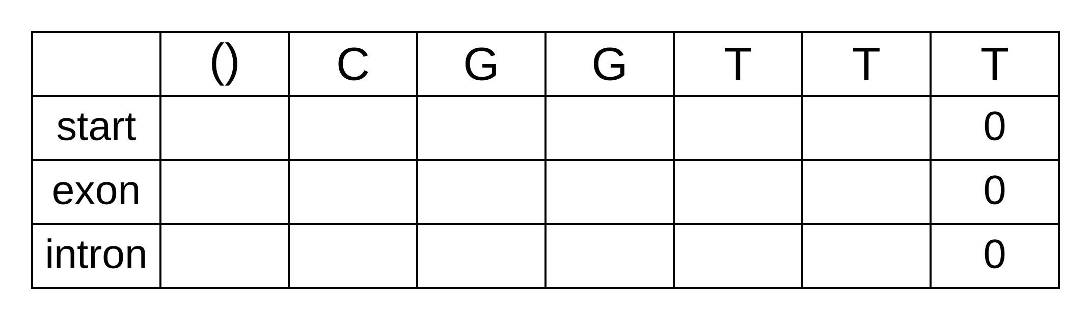
<p>To demonstrate the backward algorithm, we will use the same example sequence
CGGTTT and the same HMM as for the Viterbi and forward algorithm. Here again
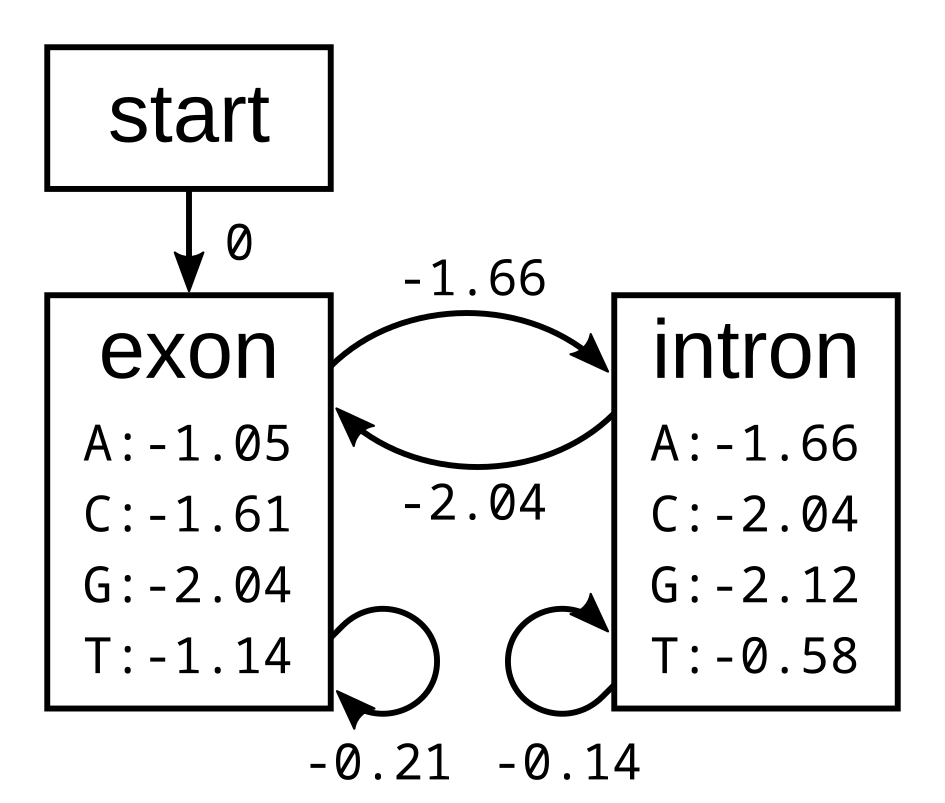
is the HMM with log emission and transmission probabilities:</p>

<p><img src="https://cs.rice.edu/~ogilvie/assets/simple-exon-intron-model-log.png" alt="Exon-intron HMM" /></p>

<p>To calculate the backward probabilities, initialize a matrix <em>b</em> of the same
dimensions as the corresponding Viterbi or forward matrices. The conditional
probability of an empty sequence after the last position is 100% (or a
log probability of zero) regardless of the state at the last position, so fill
in zeros for all states at the last column:</p>

<p><img src="https://cs.rice.edu/~ogilvie/assets/backward-0.png" alt="Initialized backwards matrix" /></p>

<p>To calculate the backward probabilities for a given hidden state <em>k</em> at the
second-to-last position <em>i</em> = <em>n</em> - 1, gather the following log probabilities
for each hidden state <em>k’</em> at position <em>i</em> + 1 = <em>n</em>:</p>

<ol>
  <li>the hidden state transition probability t<sub><em>k</em>,<em>k’</em></sub> from state <em>k</em> at <em>i</em> to state <em>k’</em> at <em>i</em> + 1</li>
  <li>the emission probability e<sub><em>k’</em>,<em>i</em>+1</sub> of the observed state (character) at <em>i</em> + 1 given <em>k’</em></li>
  <li>the probability <em>b</em><sub><em>k’</em>,<em>i</em>+1</sub> of the sequence after <em>i</em> + 1 given state <em>k’</em> at <em>i</em> + 1</li>
</ol>

<p>The sum of the above log probabilities gives us the log joint probability of
the sequence from position <em>i</em> + 1 onwards <strong>and</strong> the hidden state at <em>i</em> + 1
being <em>k’</em>, conditional on the hidden state at <em>i</em> being <em>k</em>. The log sum of
exponentials (LSE) of the log joint probabilities for each value of <em>k’</em>
marginalizes over the hidden state at <em>i</em> + 1, therefore the result of the LSE
function is the log conditional probability of the sequence alone from <em>i</em> + 1.</p>

<p>We do not have to consider transitions <em>to</em> the start state, because (1) these
transitions are not allowed by the model, and (2) there are no emission
probabilities associated with the start state. The only valid transition
<em>from</em> the start state at the second-to-last position is to an exon state, so
its log probability will be:</p>

<ul>
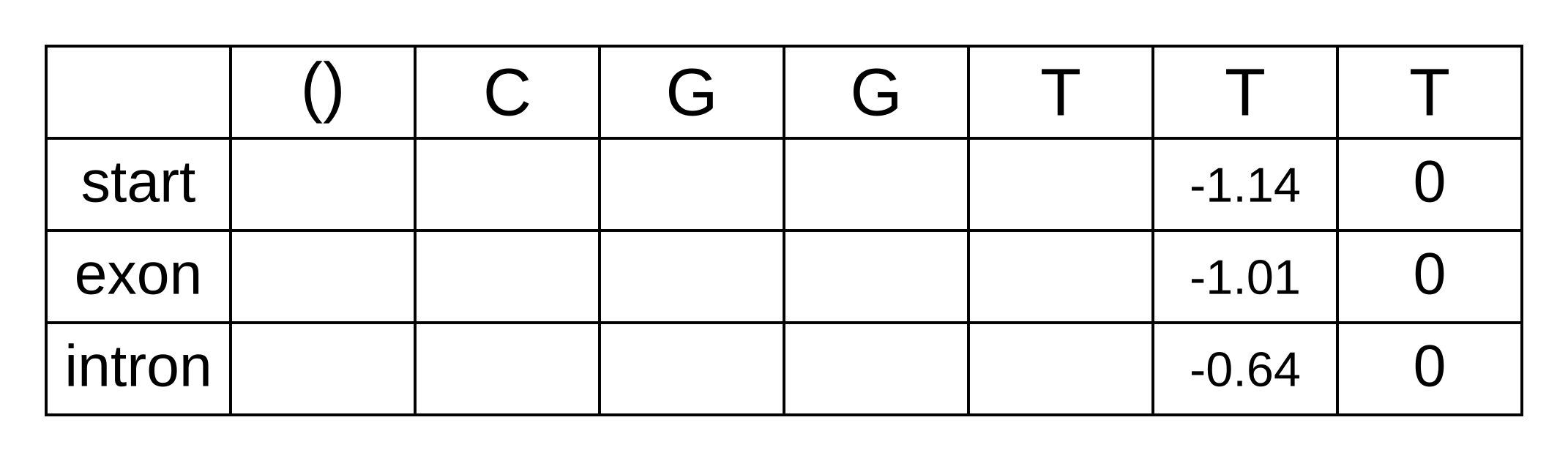
  <li><em>b</em><sub>start,<em>n</em>-1</sub> = <em>t</em><sub>start,exon</sub> + <em>e</em><sub>exon,<em>n</em></sub> + <em>b</em><sub>exon,<em>n</em></sub> = 0 + -1.14 + 0 = -1.14</li>
</ul>

<p>For the exon state at <em>n</em> - 1, we have to consider transitions to the exon or
intron states at <em>n</em>. Its log probability will be the LSE of:</p>

<ul>
  <li><em>t</em><sub>exon,exon</sub> + <em>e</em><sub>exon,<em>n</em></sub> + <em>b</em><sub>exon,<em>n</em></sub> = -0.21 + -1.14 + 0 = -1.35</li>
  <li><em>t</em><sub>exon,intron</sub> + <em>e</em><sub>intron,<em>n</em></sub> + <em>b</em><sub>intron,<em>n</em></sub> = -1.66 + -0.58 + 0 = -2.24</li>
</ul>

<p>The LSE of -1.35 and -2.24 is -1.01. and and For the intron state at <em>n</em> - 1 the log-probabilities to marginalize over are:</p>

<ul>
  <li><em>t</em><sub>intron,exon</sub> + <em>e</em><sub>exon,<em>n</em></sub> + <em>b</em><sub>exon,<em>n</em></sub> = -2.04 + -1.14 + 0 = -3.18</li>
  <li><em>t</em><sub>intron,intron</sub> + <em>e</em><sub>intron,<em>n</em></sub> + <em>b</em><sub>intron,<em>n</em></sub> = -0.14 + -0.58 + 0 = -0.72</li>
</ul>

<p>The LSE of -3.18 and -0.72 is -0.64. We can now update the backward matrix
with the second-to-last column:</p>

<p><img src="https://cs.rice.edu/~ogilvie/assets/backward-1.png" alt="Initialized backwards matrix" /></p>

<p>The third-to-last position is similar. For the start state we only have
consider the one transition permitted by the model:</p>

<ul>
  <li><em>b</em><sub>start,<em>n</em>-2</sub> = <em>t</em><sub>start,exon</sub> + <em>e</em><sub>exon,<em>n - 1</em></sub> + <em>b</em><sub>exon,<em>n - 1</em></sub> = 0 + -1.14 + -1.01 = -2.15</li>
</ul>

<p>For the exon state at <em>n</em> - 2, the same as for <em>n</em> - 1, we have to consider
two log-probabilities:</p>

<ul>
  <li><em>t</em><sub>exon,exon</sub> + <em>e</em><sub>exon,<em>n - 1</em></sub> + <em>b</em><sub>exon,<em>n - 1</em></sub> = -0.21 + -1.14 + -1.01 = -2.36</li>
  <li><em>t</em><sub>exon,intron</sub> + <em>e</em><sub>intron,<em>n - 1</em></sub> + <em>b</em><sub>intron,<em>n - 1</em></sub> = -1.66 + -0.58 + -0.64 = -2.88</li>
</ul>

<p>The LSE for these log probabilities is -1.89. Likewise for the intron state at
<em>n</em> - 2:</p>

<ul>
  <li><em>t</em><sub>intron,exon</sub> + <em>e</em><sub>exon,<em>n - 1</em></sub> + <em>b</em><sub>exon,<em>n - 1</em></sub> = -2.04 + -1.14 + -1.01 = -4.19</li>
  <li><em>t</em><sub>intron,intron</sub> + <em>e</em><sub>intron,<em>n - 1</em></sub> + <em>b</em><sub>intron,<em>n - 1</em></sub> = -0.14 + -0.58 + -0.64 = -1.36</li>
</ul>

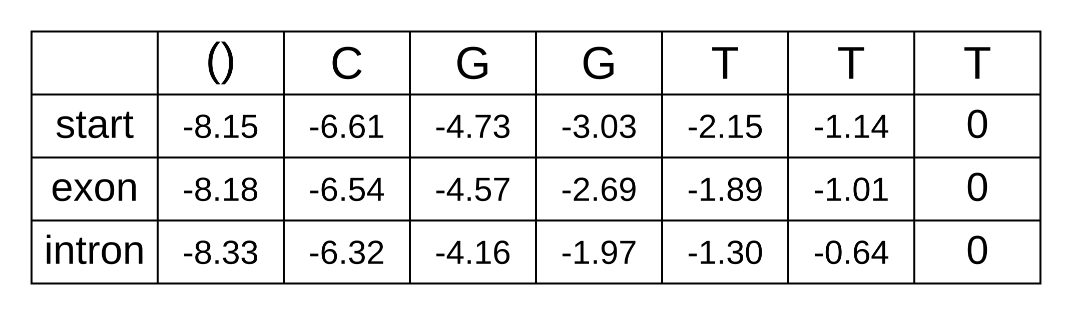
<p>And the LSE for these log probabilities is -1.30. We can now fill in the
third-to-last column of the matrix, and every column going back to the first
column of the matrix:</p>

<p><img src="https://cs.rice.edu/~ogilvie/assets/backward-2.png" alt="Initialized backwards matrix" /></p>

<p>The first column of the matrix represents the beginning of the sequence,
before any characters have been observed. The only valid hidden state for the
beginning is the start state, and therefore the log probability
<em>b</em><sub>start,0</sub> = logP(x<sub>1..<em>n</em></sub>|π<sub>0</sub>=start,M) can be
simplified to logP(x<sub>1..<em>n</em></sub>|M). Because the sequence from 1 to <em>n</em>
is the entire sequence, it can be further simplified to logP(x|M). In other
words, this value is our log marginal likelihood! Reassuringly, it is the
exact same value we previously derived using the <a href="/~ogilvie/~ogilvie/comp571/forward-algorithm/">forward algorithm</a>.</p>

<p>Why do we need two dynamic programming algorithms to compute the marginal
likelihood? We don’t! But by combining probabilities from the two matrices, we
can derive the posterior probability of each hidden state <em>k</em> at each position
<em>i</em>, marginalized over all paths through <em>k</em> at <em>i</em>. How this this work?
If two variables <em>a</em> and <em>b</em> are independent, their joint probability
P(<em>a</em>,<em>b</em>) is simply the product of their probabilities P(<em>a</em>) × P(<em>b</em>). Under
our model, the two segments of the sequence x<sub>1..<em>i</em></sub> and
x<sub><em>i</em>+1..<em>n</em></sub> are dependent on paths of hidden states. However, the
because we are using a hidden Markov model, the path and sequence from <em>i</em>
onwards  depends only on the particular hidden state at <em>i</em>. This is because
the transition probabilities are Markovian so they depend only on the previous
hidden state, and because the emission probabilities depend only on the
current hidden state. As a result, while P(x<sub>1..<em>i</em></sub>|M) and
P(x<sub><em>i</em>+1..<em>n</em></sub>|M) are not independent,
P(x<sub>1..<em>i</em></sub>|π<sub><em>i</em></sub>=<em>k</em>,M) and
P(x<sub><em>i</em>+1..<em>n</em></sub>|π<sub><em>i</em></sub>=<em>k</em>,M) are! Therefore (dropping
the model term M for space and clarity):</p>

<p>P(x<sub>1..<em>i</em></sub>|π<sub><em>i</em></sub>=<em>k</em>) × P(x<sub><em>i</em>+1..<em>n</em></sub>|π<sub><em>i</em></sub>=<em>k</em>) × P(π<sub><em>i</em></sub>=<em>k</em>) = P(x<sub>1..<em>i</em></sub>, x<sub><em>i</em> + 1..<em>n</em></sub>|π<sub><em>i</em></sub>=<em>k</em>) × P(π<sub><em>i</em></sub>=<em>k</em>) = P(x|π<sub><em>i</em></sub>=<em>k</em>) × P(π<sub><em>i</em></sub>=<em>k</em>)</p>

<p>Using the transitivity of equivalence, the product on the left hand side above
must equal the product on the right hand side above. By applying the <a href="https://en.wikipedia.org/wiki/Chain_rule_(probability)">chain
rule</a>, it can also be shown that both are equal to the product on the right
hand side below:</p>

<p>P(x|π<sub><em>i</em></sub>=<em>k</em>) × P(π<sub><em>i</em></sub>=<em>k</em>) = P(x<sub>1..<em>i</em></sub>|π<sub><em>i</em></sub>=<em>k</em>) × P(x<sub><em>i</em>+1..<em>n</em></sub>|π<sub><em>i</em></sub>=<em>k</em>) × P(π<sub><em>i</em></sub>=<em>k</em>) = P(x<sub>1..<em>i</em></sub>, π<sub><em>i</em></sub>=<em>k</em>) × P(x<sub><em>i</em>+1..<em>n</em></sub>|π<sub><em>i</em></sub>=<em>k</em>)</p>

<p>Or in log space:</p>

<p>logP(x|π<sub><em>i</em></sub>=<em>k</em>) + logP(π<sub><em>i</em></sub>=<em>k</em>) = logP(x<sub>1..<em>i</em></sub>, π<sub><em>i</em></sub>=<em>k</em>) + logP(x<sub><em>i</em>+1..<em>n</em></sub>|π<sub><em>i</em></sub>=<em>k</em>)</p>

<p>Notice that the sum on the right hand side above corresponds exactly to
<em>f</em><sub><em>k</em>,<em>i</em></sub> + <em>b</em><sub><em>k</em>,<em>i</em></sub>! Now using Bayes rule, and
remembering that <em>b</em><sub>start,0</sub> equals the log marginal likelihood, we
can calculate the log posterior probability of π<sub><em>i</em></sub>=<em>k</em>:</p>

<p>logP(π<sub><em>i</em></sub>=<em>k</em>|x) = logP(x|π<sub><em>i</em></sub>=<em>k</em>) + logP(π<sub><em>i</em></sub>=<em>k</em>) - logP(x) = logP(x<sub>1..<em>i</em></sub>, π<sub><em>i</em></sub>=<em>k</em>) + logP(x<sub><em>i</em>+1..<em>n</em></sub>|π<sub><em>i</em></sub>=<em>k</em>) - logP(x) = <em>f</em><sub><em>k</em>,<em>i</em></sub> + <em>b</em><sub><em>k</em>,<em>i</em></sub> - <em>b</em><sub><em>0</em>,<em>start</em></sub></p>

<p>And now we can now “decode” our posterior distribution of hidden states. We need to refer
back to the previously calculated forward matrix, shown below.</p>

<p><img src="https://cs.rice.edu/~ogilvie/assets/forward-2.png" alt="Previously calculated forward matrix" /></p>

<p>As an example, let’s solve the log marginal probability that the hidden state
of the fourth character is an exon:</p>

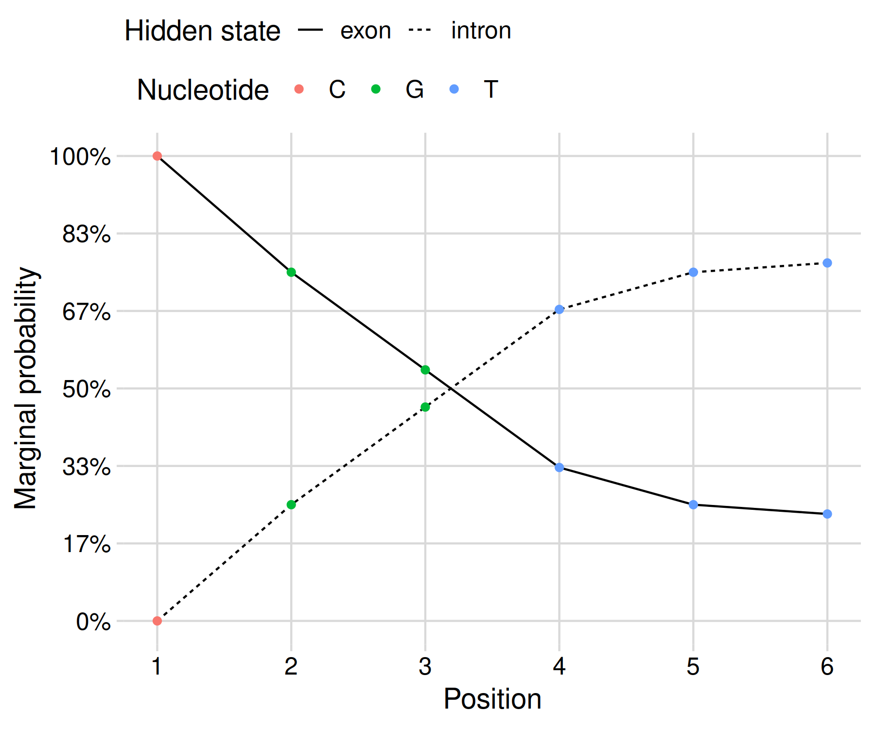
<p>logP(π<sub>4</sub>=<em>exon</em>|x,M) = <em>f</em><sub><em>exon</em>,4</sub> + <em>b</em><sub><em>exon</em>,4</sub> - <em>b</em><sub>start,0</sub> = -1.89 + -7.36 - -8.15 = -1.1</p>

<p>The marginal probability is exp(-1.1) = 33%. Since we only have two states,
the probability of the intron state should be 67%, but let’s double check to
make sure:</p>

<p>logP(π<sub>4</sub>=<em>intron</em>|x,M) = <em>f</em><sub><em>intron</em>,4</sub> + <em>b</em><sub><em>intron</em>,4</sub> - <em>b</em><sub>start,0</sub> = -1.30 + -7.25 - -8.15 = -0.4</p>

<p>Since exp(-0.4) = 67%, it seems like we are on the right track! The posterior
probabilities can be shown as a graph in order to clearly communicate your
results:</p>

<p><img src="https://cs.rice.edu/~ogilvie/assets/exon-intron-decoded.png" alt="Exon-intron posterior decoding" /></p>

<p>This gives us a result that reflects the uncertainty of our inference given
the limited data at hand. In my opinion, this presentation is more honest than
the black-and-white maximum <em>a posteriori</em> result derived using Viterbi’s
algorithm.</p>

<p>For another perspective on the backward algorithm, consult lesson 10.11 of <a href="https://www.bioinformaticsalgorithms.org/bioinformatics-chapter-10">Bioinformatics Algorithms</a> by Compeau and Pevzner.</p>]]></content><author><name>Huw A. Ogilvie</name></author><category term="comp571" /><summary type="html"><![CDATA[Like the forward algorithm, we can use the backward algorithm to calculate the marginal likelihood of a hidden Markov model (HMM). Also like the forward algorithm, the backward algorithm is an instance of dynamic programming where the intermediate values are probabilities.]]></summary></entry><entry><title type="html">Forward algorithm</title><link href="https://cs.rice.edu/~ogilvie/comp571/forward-algorithm/" rel="alternate" type="text/html" title="Forward algorithm" /><published>2020-10-23T01:00:00-05:00</published><updated>2020-10-23T01:00:00-05:00</updated><id>https://cs.rice.edu/~ogilvie/comp571/forward-algorithm</id><content type="html" xml:base="https://cs.rice.edu/~ogilvie/comp571/forward-algorithm/"><![CDATA[<p>The <a href="/~ogilvie/~ogilvie/comp571/viterbi-algorithm/">Viterbi algorithm</a> identifies a single path of hidden Markov model
(HMM) states. This is the path which maximizes the joint probability of the
observed data (e.g. a nucleotide or amino acid sequence) and the hidden
states, given the HMM (including transition and emission frequencies).</p>

<p>Maybe this path is almost certainly correct, but it also might represent one
of many plausible paths. Putting things quantitatively, the Viterbi result
might have a 99.9% probability of being the true<sup id="fnref:1" role="doc-noteref"><a href="#fn:1" class="footnote" rel="footnote">1</a></sup> path, or a 0.1%
probability. It would be useful to know these probabilities in order to
understand when our results obtained from the Viterbi algorithm are reliable.</p>

<p>Recall that the joint probability is P(π,x|M) where (in the context of
biological sequence analysis) x is the biological sequence, π is the state
path, and M is the HMM. Following the <a href="https://en.wikipedia.org/wiki/Chain_rule_(probability)">chain rule</a>, this is equivalent to
P(x|π,M) × P(π|M). The maximum joint probability returned by the Viterbi
algorithm is therefore the product of the <a href="/~ogilvie/~ogilvie/comp571/probability-and-likelihood-distributions/">likelihood</a> of the sequence
given the state path, and the prior probability of the state path! Previously
I have described the product of the likelihood and prior as the <a href="/~ogilvie/~ogilvie/comp571/bayesian-inference/">unnormalized
posterior probability</a>. The parameter values which maximize that product,
and therefore the state path returned by the Viterbi algorithm, is often
known as the “maximum <em>a posteriori</em>” solution.</p>

<p>The posterior probability is obtained by dividing the unnormalized posterior
probability (which can be obtained using the Viterbi algorithm) by the
marginal likelihood. The marginal likelihood can be calculated using the
<strong>forward algorithm</strong>.</p>

<p>The intermediate probabilities calculated using the Viterbi algorithm are the
probabilities of a state path π and a biological sequence x up to some step
<em>i</em>: P(π<sub>1..i</sub>,x<sub>1..i</sub>|M). The intermediate probabilities
calculated using the forward algorithm are similar but marginalize over the
state path up to step <em>i</em>: P(π<sub>i</sub>,x<sub>1..i</sub>|M). Put another
way, the probability is for the state at position <em>i</em> integrated over the path
followed to that state.</p>

<p>This marginalization is achieved by summing over the choices made at each
step. When calculating probabilities, summing typically achieves the result of
X <strong>or</strong> Y (e.g., a high OR low path), whereas a product typically achieves
the result of X <strong>and</strong> Y (e.g. a high then low path).</p>

<p>Just as for the Viterbi algorithm, it is sensible to work in log space to
avoid numerical underflows and loss of precision. As an alternative to working
in log space while still avoiding those errors, the marginal probabilities of
all states at any position along the sequence can be rescaled (see section
3.6 of <a href="https://www.amazon.com/Biological-Sequence-Analysis-Probabilistic-Proteins/dp/0521629713">Biological Sequence Analysis</a>). However if those marginal
probabilities are very different in magnitude, there can still be numerical
errors even with rescaling, so from here on we will work in log space.</p>

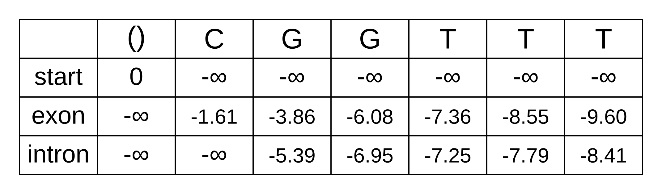
<p>As an example we will use the forward algorithm to calculate the log marginal
likelihood of the sequence <code class="language-plaintext highlighter-rouge">CGGTTT</code> and HMM used in the <a href="/~ogilvie/~ogilvie/comp571/viterbi-algorithm/">Viterbi example</a>.
Initialize an empty forward matrix with the first row and column filled in,
same as the Viterbi matrix:</p>

<p><img src="https://cs.rice.edu/~ogilvie/assets/forward-0.png" alt="Initialized forward matrix" /></p>

<p>To calculate the log marginal probability of a particular state at some
position of the sequence, we need to sum over the probabilies that lead from
any previous state to the particular state at that position. These are <strong>not</strong>
the log-probabilities being summed over, but the actual zero to one
probabilities. In log space, this requires logging the sum of exponentials
of the log-probabilities, or <a href="https://en.wikipedia.org/wiki/LogSumExp">LogSumExp</a> (LSE) for short.</p>

<p>The only valid paths up to the second position of the sequence under our model
are start-exon-exon and start-exon-intron, so the first three columns will be
identical to the Viterbi matrix as no summation is required:</p>

<p><img src="https://cs.rice.edu/~ogilvie/assets/forward-1.png" alt="First three columns filled in" /></p>

<p>Because of the marginalization, there are no pointer arrows to add to the
forward matrix. The third position (fourth column) is more interesting, as we
have to marginalize over multiple log probabilities of the state at the
previous position. For the exon state at the third position, these log
probabilities <a href="/~ogilvie/~ogilvie/comp571/viterbi-algorithm/">are</a>:</p>

<ul>
  <li><em>f</em><sub>exon,2</sub> + <em>t</em><sub>exon,exon</sub> + <em>e</em><sub>exon,3</sub> = -3.86 + -0.21 + + -2.04 = -6.11</li>
  <li><em>f</em><sub>intron,2</sub> + <em>t</em><sub>intron,exon</sub> + <em>e</em><sub>exon,3</sub> = -5.39 + -2.04 + -2.04 = -9.47</li>
</ul>

<p>The log marginal probability (to two decimal places) is therefore LSE(-6.11,
-9.47) = log(exp(-6.11) + exp(-9.47)) = -6.08. This calculation can be
performed in one step using the Python function <code class="language-plaintext highlighter-rouge">scipy.special.logsumexp</code>. To
use this command <a href="http://scipy.org/">scipy</a> must be installed and the <code class="language-plaintext highlighter-rouge">scipy.special</code>
subpackage must be imported. In fact, it should be performed in one step to
avoid the aforementioned numerical errors.</p>

<p>The log probabilities to marginalize over for the intron state at the third
position <a href="/~ogilvie/~ogilvie/comp571/viterbi-algorithm/">are</a>:</p>

<ul>
  <li><em>f</em><sub>exon,2</sub> + <em>t</em><sub>exon,intron</sub> + <em>e</em><sub>intron,3</sub> = -3.86 + -1.66 + -2.12 = -7.64</li>
  <li><em>f</em><sub>intron,2</sub> + <em>t</em><sub>intron,intron</sub> + <em>e</em><sub>intron,3</sub> = -5.39 + -0.14 + -2.12 = -7.65</li>
</ul>

<p>The log marginal probability is therefore LSE(-7.64, -7.65) = log(exp(-7.64) +
exp(-7.65)) = -6.95. The log marginal probabilities for each state at each
position can be calculated the same way, and the completed forward matrix will
be:</p>

<p><img src="https://cs.rice.edu/~ogilvie/assets/forward-2.png" alt="First three columns filled in" /></p>

<p>At the last position, we have the log marginal joint probability of the
sequence and path over all paths that end in an exon state, and log marginal
joint probability over all paths that end in an intron state. The LSE of these
two log probabilities is therefore the log marginal likelihood of the model,
because it marginalizes over all state paths, and equals to LSE(-9.60, -8.41)
= log(exp(-9.60) + exp(-8.41)) = -8.15.</p>

<p>We previously calculated the log probability of the maximum <em>a posteriori</em>
path as -9.79. The posterior probability is therefore exp(-9.79 - -8.15) =
exp(-1.64) = 19.4%. The Viterbi result is very plausible (events with 19.4%
probability occur all the time) but most likely wrong.</p>

<p>For more information see section 3.2 of <a href="https://www.amazon.com/Biological-Sequence-Analysis-Probabilistic-Proteins/dp/0521629713">Biological Sequence analysis</a> by
Durbin, Eddy, Krogh and Mitchison.</p>

<p>For another perspective on the forward algorithm, consult lesson 10.7 of <a href="https://www.bioinformaticsalgorithms.org/bioinformatics-chapter-10">Bioinformatics Algorithms</a> by Compeau and Pevzner.</p>

<div class="footnotes" role="doc-endnotes">
  <ol>
    <li id="fn:1" role="doc-endnote">
      <p>Such probabilities are conditioned on the model being correct. So more accurately, they are the probability of a parameter value being true if the model (e.g. an HMM) used for inference is also the model which generated the data. If the model is wrong, the probabilities can be quite spurious, see <a href="https://arxiv.org/abs/1810.05398">Yang and Zhu (2018)</a>. <a href="#fnref:1" class="reversefootnote" role="doc-backlink">&#8617;</a></p>
    </li>
  </ol>
</div>]]></content><author><name>Huw A. Ogilvie</name></author><category term="comp571" /><summary type="html"><![CDATA[The Viterbi algorithm identifies a single path of hidden Markov model (HMM) states. This is the path which maximizes the joint probability of the observed data (e.g. a nucleotide or amino acid sequence) and the hidden states, given the HMM (including transition and emission frequencies).]]></summary></entry><entry><title type="html">Viterbi algorithm</title><link href="https://cs.rice.edu/~ogilvie/comp571/viterbi-algorithm/" rel="alternate" type="text/html" title="Viterbi algorithm" /><published>2020-10-22T09:00:00-05:00</published><updated>2020-10-22T09:00:00-05:00</updated><id>https://cs.rice.edu/~ogilvie/comp571/viterbi-algorithm</id><content type="html" xml:base="https://cs.rice.edu/~ogilvie/comp571/viterbi-algorithm/"><![CDATA[<p>The Viterbi algorithm is used to efficiently infer the most probable “path” of
the unobserved random variable in an HMM. In the CpG islands case, this is the
most probable combination of CG-rich and CG-poor states over the length of the
sequence. In the splicing case, this the most probable structure of the gene in
terms of exons and introns.</p>

<p>Conceptually easier than Viterbi would be the brute force solution of
calculating the probability for all possible paths. However the number of
possible paths for two states, as in the CpG island model, is 2<sup><em>n</em></sup>
where <em>n</em> is the number of sites. For even a short sequence of 1000
nucleotides, this equates to 2<sup>1000</sup> paths, or approximately
10<sup>301</sup>. This number is about 10<sup>221</sup> times larger than
<a href="https://physics.stackexchange.com/a/68346">the number of atoms in the observable universe</a>.</p>

<p>I will first demonstrate how the algorithm works using the following simple
exon-intron model:</p>

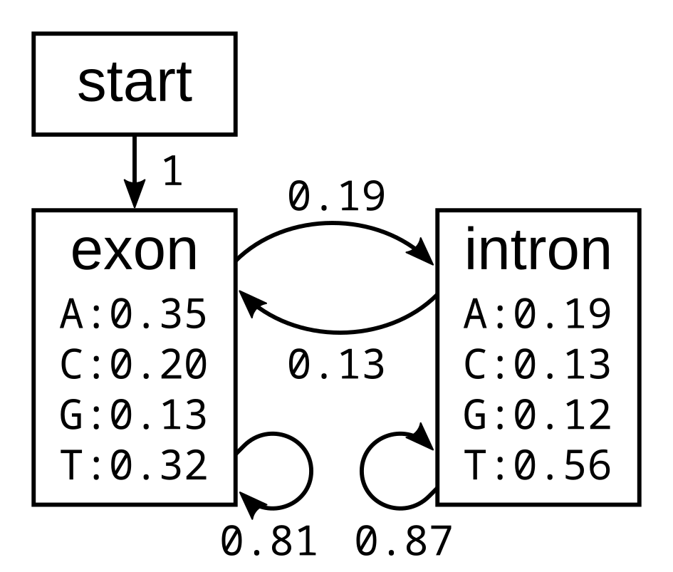
<p><img src="https://cs.rice.edu/~ogilvie/assets/simple-exon-intron-model.png" alt="Simple exon intron model" /></p>

<p>The probabilities of the model have the corresponding log-probabilities, to
two decimal places:</p>

<p><img src="https://cs.rice.edu/~ogilvie/assets/simple-exon-intron-model-log.png" alt="Corresponding log-probabilities" /></p>

<p>Let’s apply this simple model to the toy sequence CGGTTT.</p>

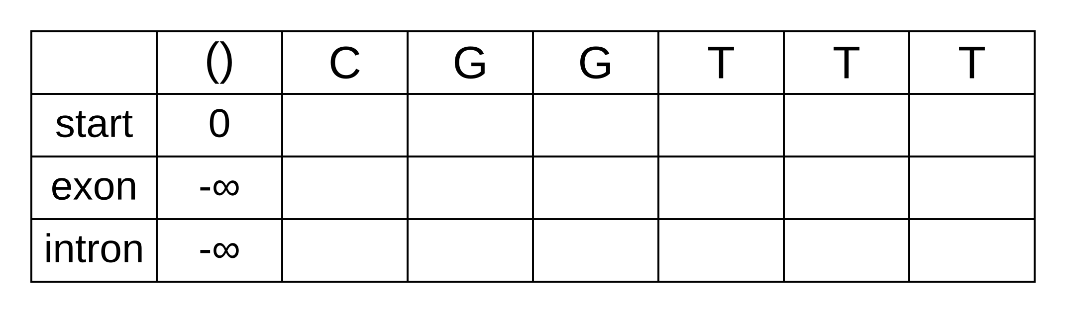
<p>Draw up a table and fill in the probabilities of the states when the sequence
is empty: 0 log-probability (100% probability) for being in the start state at the
start of the sequence, and negative infinity (0% probability) for not being in the
start state at the start of the sequence:</p>

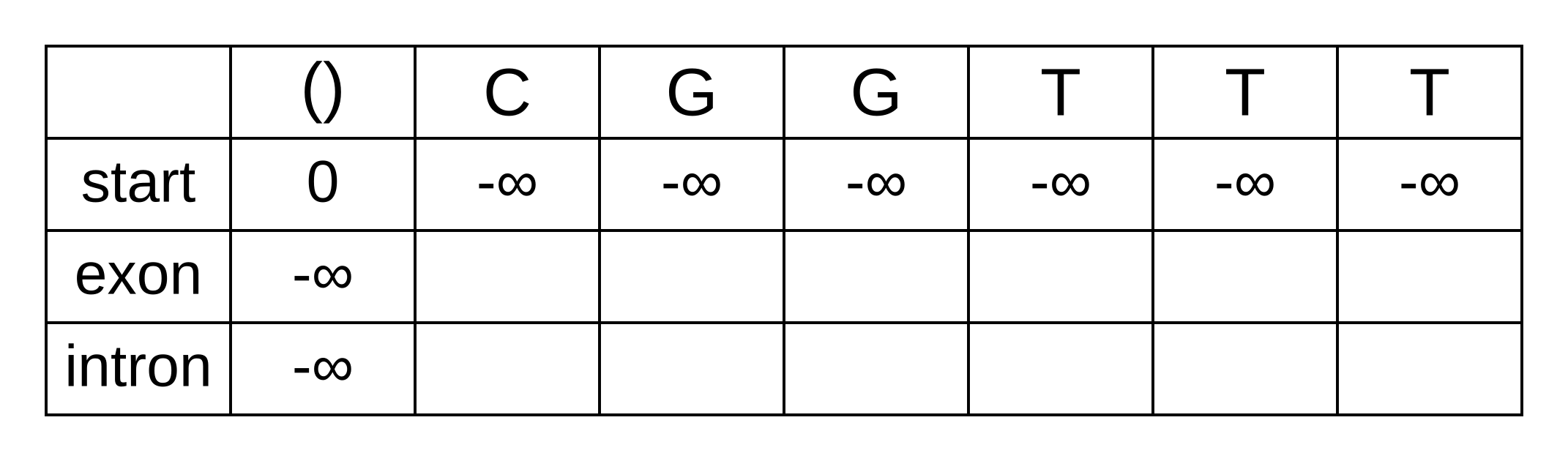
<p><img src="https://cs.rice.edu/~ogilvie/assets/viterbi-0.png" alt="Viterbi with first column filled in" /></p>

<p>We will refer to every element of the matrix as v<sub><em>k,i</em></sub> where <em>k</em> is
the hidden state, and <em>i</em> is the position within the sequence.
v<sub><em>k,i</em></sub> is the maximum log joint probability of the sequence and any path up
to <em>i</em> where the hidden state at <em>i</em> is <em>k</em>:</p>

<p>v<sub><em>k,i</em></sub> = max<sub>path<sub>1..<em>i</em>-1</sub></sub>(logP(seq<sub>1..<em>i</em></sub>, path<sub>1..<em>i</em>-1</sub>, path<sub><em>i</em></sub> = <em>k</em>)).</p>

<p>This log joint probability is equal to the maximum value of
v<sub><em>k’</em>,<em>i</em>-1</sub> where <em>k’</em> is the hidden state at the previous
position, plus the transition log-probability t<sub><em>k’</em>,<em>k</em></sub> of
transitioning from the state <em>k’</em> to <em>k</em>, plus the emission log-probability
e<sub><em>k,i</em></sub> of the nucleotide (or amino acid for proteins) at <em>i</em> given
<em>k</em>. We find this value by calculating this sum for every previous
hidden state <em>k’</em> and choosing the maximum.</p>

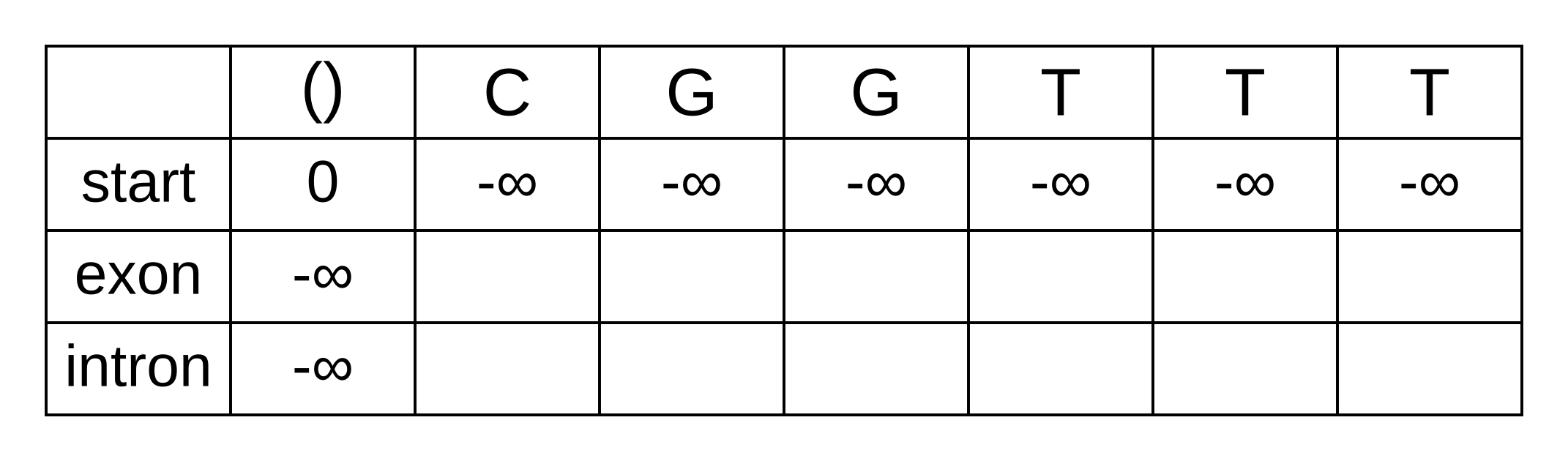
<p>The transition log probability from any state to the start state is -∞, so for
any value of <em>i</em> from 1 onwards, v<sub>start,<em>i</em></sub> = -∞. Go ahead and fill
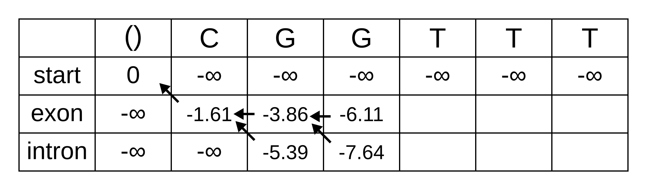
those in to save time:</p>

<p><img src="https://cs.rice.edu/~ogilvie/assets/viterbi-1.png" alt="Viterbi with first row filled in" /></p>

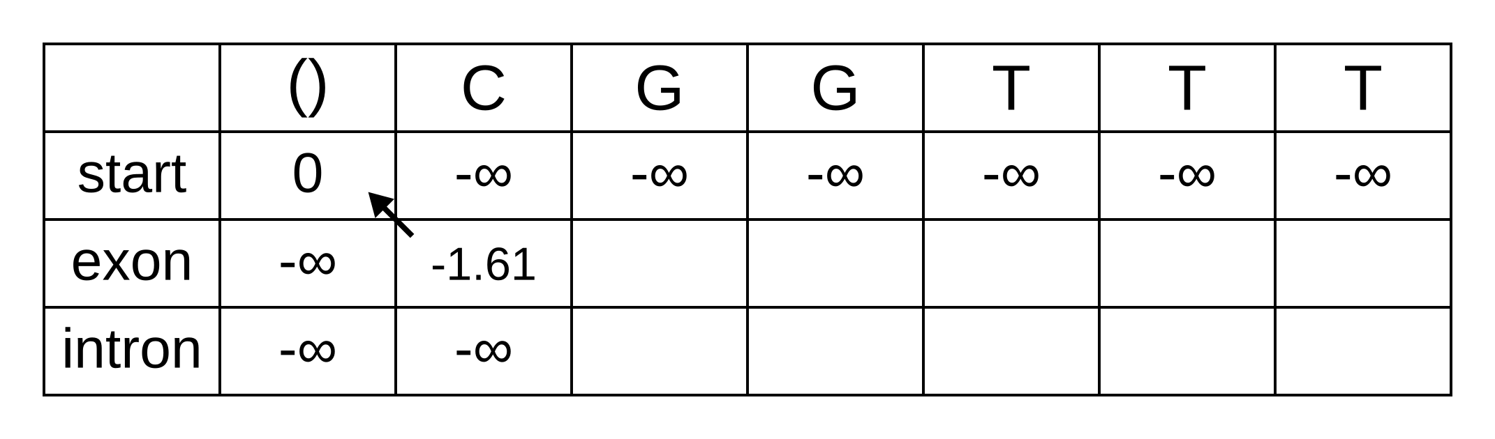
<p>For the next element v<sub>exon,1</sub> we only have to consider the
transition from the start state to the exon state, because that is the only
transition permitted by the model. Even if we do the calculations for the
other transitions, the results of those calculations will be negative infinities
because the Viterbi probability of non-start states in the first column are
negative infinities. The log-probability at v<sub>exon,1</sub> is therefore:</p>

<ul>
  <li><em>v</em><sub>exon,1</sub> = <em>v</em><sub>start,0</sub> + <em>t</em><sub>start,exon</sub> + <em>e</em><sub>exon,1</sub> = 0 + 0 + -1.61 = -1.61</li>
</ul>

<p>The log-probability of <em>v</em><sub>intron,1</sub> is negative infinity because the
model does not permit the state at the first sequence position to be an
intron. This can be effected computationally by setting the
<em>t</em><sub>start,intron</sub> log-probability to negative infinity. Then
regardless of the Viterbi and emission log-probabilities, the sum of <em>v</em>, <em>t</em>
and <em>e</em> will be negative infinity.</p>

<p>Fill in both values for the first position of the sequence (or second column
of the matrix), and add a pointer from the exon state to the start state:</p>

<p><img src="https://cs.rice.edu/~ogilvie/assets/viterbi-2.png" alt="Viterbi with first position filled in" /></p>

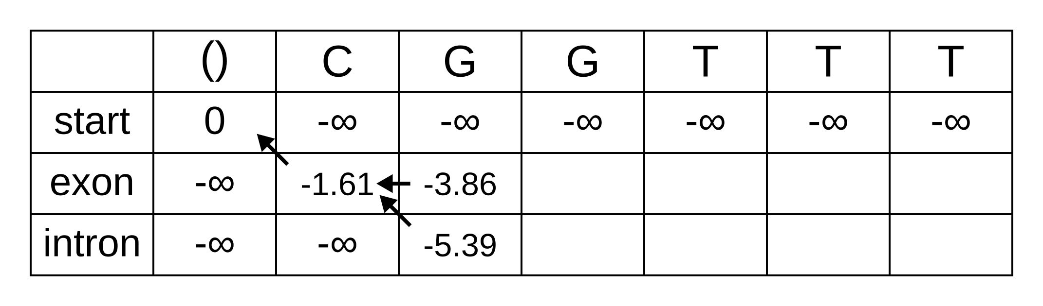
<p>Once we get to <em>v</em><sub>exon,2</sub>, we only have to consider the exon to exon
transition since the log-probabilities for the other states at the previous
position are negative infinities. So this log-probability will be:</p>

<ul>
  <li><em>v</em><sub>exon,2</sub> = <em>v</em><sub>exon,1</sub> + <em>t</em><sub>exon,exon</sub> + <em>e</em><sub>exon,2</sub> = -1.61 + -0.21 + -2.04 = -3.86</li>
</ul>

<p>And for the same reason to calculate <em>v</em><sub>intron,2</sub> we only have to
consider the exon to intron transition, and this log-probability will be:</p>

<ul>
  <li><em>v</em><sub>intron,2</sub> = <em>v</em><sub>exon,1</sub> + <em>t</em><sub>exon,intron</sub> + <em>e</em><sub>intron,2</sub> = -1.61 + -1.66 + -2.12 = -5.39</li>
</ul>

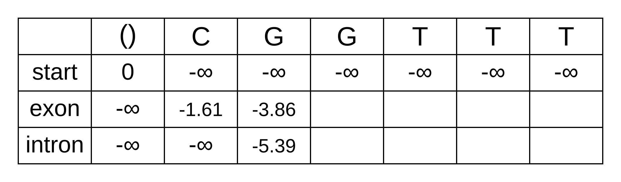
<p>So fill on those values, and add pointers to the only permitted previous state,
which is the exon state:</p>

<p><img src="https://cs.rice.edu/~ogilvie/assets/viterbi-3.png" alt="Viterbi with second position filled in" /></p>

<p>For the next position, we have to consider all transitions between intron or
exon to intron or exon since both of those states have finite
log-probabilities at the previous position. The log-probability of
<em>v</em><sub>exon,3</sub> will be the maximum of:</p>

<ul>
  <li><em>v</em><sub>exon,2</sub> + <em>t</em><sub>exon,exon</sub> + <em>e</em><sub>exon,3</sub> = -3.86 + -0.21 + -2.04 = -6.11</li>
  <li><em>v</em><sub>intron,2</sub> + <em>t</em><sub>intron,exon</sub> + <em>e</em><sub>exon,3</sub> = -5.39 + -2.04 + -2.04 = -9.47</li>
</ul>

<p>The previous hidden state that maximizes the Viterbi log-probability for the
exon state at the third sequence position is therefore the exon state, and
the maximum log-probability is -6.11. The log-probability of <em>v</em><sub>intron,3</sub>
will be the maximum of:</p>

<ul>
  <li><em>v</em><sub>exon,2</sub> + <em>t</em><sub>exon,intron</sub> + <em>e</em><sub>intron,3</sub> = -3.86 + -1.66 + -2.12 = -7.64</li>
  <li><em>v</em><sub>intron,2</sub> + <em>t</em><sub>intron,intron</sub> + <em>e</em><sub>intron,3</sub> = -5.39 + -0.14 + -2.12 = -7.65</li>
</ul>

<p>The previous hidden state that maximizes the Viterbi log-probability for the
intron state at the third sequence position is therefore also the exon state,
and the maximum log-probability is -7.64.</p>

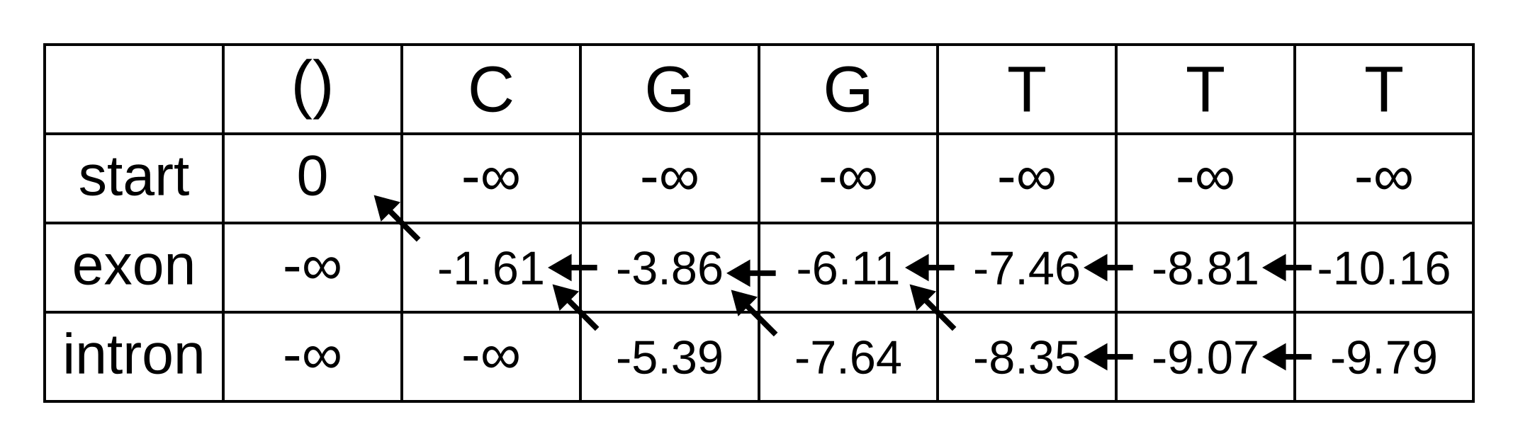
<p>Fill in the maximum log-probabilities for each hidden state <em>k</em>, and also draw
pointers to the previous hidden states corresponding to those maximum
log-probabilities:</p>

<p><img src="https://cs.rice.edu/~ogilvie/assets/viterbi-4.png" alt="Completed Viterbi matrix" /></p>

<p>The rest of the matrix is filled in the same way as for the third position:</p>

<p><img src="https://cs.rice.edu/~ogilvie/assets/viterbi-5.png" alt="Completed Viterbi matrix" /></p>

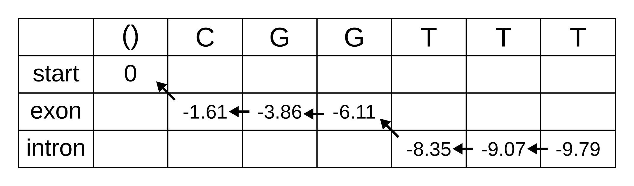
<p>The maximum log joint probability of the sequence and path is the maximum out of
v<sub><em>k,L</em></sub>, where <em>L</em> is the length of the sequence. In other words, if
we calculate the log joint probability</p>

<p>v<sub><em>k,L</em></sub> = max<sub>path<sub>1..<em>L</em>-1</sub></sub>(logP(seq<sub>0..<em>L</em></sub>, path<sub>0..<em>L</em>-1</sub>, path<sub><em>L</em></sub> = <em>k</em>)).</p>

<p>for every value of <em>k</em>, we can identify the maximum log joint probability
unconditional on the value of <em>k</em> at <em>L</em>. The path is then reconstructed by
following the pointers backwards from the maximum log joint probability. In
our toy example, the maximum log joint probability is -9.79 and the path is:</p>

<p><img src="https://cs.rice.edu/~ogilvie/assets/viterbi-6.png" alt="Completed Viterbi matrix" /></p>

<p>Or, ignoring the start state, exon-exon-exon-intron-intron-intron.</p>

<p>The basic Viterbi algorithm has a number of important properties:</p>

<ul>
  <li>Its space and time complexity is O(<em>Ln</em>) and O(<em>Ln</em><sup>2</sup>) respectively, where <em>n</em> is the number of states and <em>L</em> is the length of the sequence</li>
  <li>It returns a point estimate rather than a probability distribution</li>
  <li>Like Needleman–Wunsch or Smith–Waterman it is exact, so it is guaranteed to find the optimal<sup id="fnref:1" role="doc-noteref"><a href="#fn:1" class="footnote" rel="footnote">1</a></sup> solution, unlike heuristic algorithms, and unlike an MCMC chain run for a finite number of steps<sup id="fnref:2" role="doc-noteref"><a href="#fn:2" class="footnote" rel="footnote">2</a></sup></li>
  <li>The probability is the (log) <a href="/~ogilvie/~ogilvie/comp571/probability-and-likelihood-distributions/">joint</a> <a href="/~ogilvie/~ogilvie/comp571/probability-and-likelihood-distributions/">probability</a> of the <em>entire</em> sequence (e.g. nucleotides or amino acids) <strong>and</strong> the <em>entire</em> path of unobserved states. It is <em>not</em> identifying the most probable hidden state at each position, because it is not <a href="/~ogilvie/~ogilvie/comp571/probability-and-likelihood-distributions/">marginalizing</a> over the hidden states at other positions.</li>
</ul>

<p>If the joint probability is close to sum of all joint probabilities, in other
words if there are no other plausible state paths, then the point estimate
returned by the algorithm will be reliable. Let’s see how it performs for our
splice site model. The following code implements the Viterbi algorithm by
reading in a previously inferred HMM to analyze a novel sequence:</p>

<div class="language-plaintext highlighter-rouge"><div class="highlight"><pre class="highlight"><code>import csv
import numpy
import sys

neginf = float("-inf")

def read_fasta(fasta_path):
	label = None
	sequence = None

	fasta_sequences = {}

	fasta_file = open(fasta_path)

	l = fasta_file.readline()
	while l != "":
		if l[0] == "&gt;":
			if label != None:
				fasta_sequences[label] = sequence

			label = l[1:].strip()
			sequence = ""
		elif label != None:
			sequence += l.strip()

		l = fasta_file.readline()

	fasta_file.close()

	if label != None:
		fasta_sequences[label] = sequence

	return fasta_sequences

def read_matrix(matrix_path):
	matrix_file = open(matrix_path)
	matrix_reader = csv.reader(matrix_file)

	column_names = next(matrix_reader)

	list_of_numeric_rows = []
	for row in matrix_reader:
		numeric_row = numpy.array([float(x) for x in row])
		list_of_numeric_rows.append(numeric_row)

	matrix_file.close()

	matrix = numpy.stack(list_of_numeric_rows)

	return column_names, matrix

# ignore warnings caused by zero probability states
numpy.seterr(divide = "ignore")

emission_matrix_path     = sys.argv[1]
transmission_matrix_path = sys.argv[2]
fasta_path               = sys.argv[3]

sequence_alphabet, e_matrix = read_matrix(emission_matrix_path)
hidden_state_alphabet, t_matrix = read_matrix(transmission_matrix_path)

log_e_matrix = numpy.log(e_matrix)
log_t_matrix = numpy.log(t_matrix)

m = len(hidden_state_alphabet) # the number of hidden states

fasta_sequences = read_fasta(fasta_path)

for sequence_name in fasta_sequences:
	sequence = fasta_sequences[sequence_name]

	n = len(sequence) # the length of the sequence and index of the last position

	# the first character is also offset by 1, for pseudo-1-based-addressing
	numeric_sequence = numpy.zeros(n + 1, dtype = numpy.uint8)
	for i in range(n):
		numeric_sequence[i + 1] = sequence_alphabet.index(sequence[i])

	# all calculations will be in log space
	v_matrix = numpy.zeros((m, n + 1)) # Viterbi log probabilities
	p_matrix = numpy.zeros((m, n + 1), dtype = numpy.uint8) # Viterbi pointers

	# initialize matrix probabilities
	v_matrix.fill(neginf)
	v_matrix[0, 0] = 0.0

	temp_vitebri_probabilities = numpy.zeros(m)

	for i in range(1, n + 1):
		for k in range(1, m): # state at i
			for j in range(m): # state at i - 1
				e = log_e_matrix[k, numeric_sequence[i]]
				t = log_t_matrix[j, k]
				v = v_matrix[j, i - 1]

				temp_vitebri_probabilities[j] = e + t + v

			v_matrix[k, i] = numpy.max(temp_vitebri_probabilities)
			p_matrix[k, i] = numpy.argmax(temp_vitebri_probabilities)

	# initialize the maximum a posteriori hidden state path using the state with
	# the highest joint probability at the last position
	map_state = numpy.argmax(v_matrix[:, n])

	# then follow the pointers backwards from (n - 1) to 0
	for i in reversed(range(n)):
		subsequent_map_state = map_state
		map_state = p_matrix[subsequent_map_state, i + 1]

		if map_state != subsequent_map_state:
			print("Transition from %s at position %d to %s at position %d" % (hidden_state_alphabet[map_state], i, hidden_state_alphabet[subsequent_map_state], i + 1))
</code></pre></div></div>

<p>The first and second arguments for this program are paths to the emission matrix and
transmission matrix respectively. A simplified version of the emission matrix from the
<a href="/~ogilvie/~ogilvie/comp571/hidden-markov-models/">previously inferred gene structure HMM</a> looks like this:</p>

<div class="language-plaintext highlighter-rouge"><div class="highlight"><pre class="highlight"><code>A,C,G,T
0.0000,0.0000,0.0000,0.0000
0.2905,0.2018,0.2349,0.2728
0.0952,0.0327,0.7735,0.0986
0.0011,0.0000,0.9988,0.0001
0.2786,0.1581,0.1581,0.4052
0.0000,0.0010,0.9989,0.0001
0.2535,0.1039,0.5197,0.1229
</code></pre></div></div>

<p>And a simplified version of the transition matrix looks like this:</p>

<div class="language-plaintext highlighter-rouge"><div class="highlight"><pre class="highlight"><code>start,exon interior,exon 3',intron 5',intron interior,intron 3',exon 5'
0.0000,1.0000,0.0000,0.0000,0.0000,0.0000,0.0000
0.0000,0.9962,0.0038,0.0000,0.0000,0.0000,0.0000
0.0000,0.0000,0.0000,1.0000,0.0000,0.0000,0.0000
0.0000,0.0000,0.0000,0.0000,1.0000,0.0000,0.0000
0.0000,0.0000,0.0000,0.0000,0.9935,0.0065,0.0000
0.0000,0.0000,0.0000,0.0000,0.0000,0.0000,1.0000
0.0000,1.0000,0.0000,0.0000,0.0000,0.0000,0.0000
</code></pre></div></div>

<p>We can analyse the Arabidopsis gene FOLB2 (which codes for an enzyme that is
part of the folate biosynthesis pathway). Warning: this is committing the
cardinal sin of testing a model using data from the training set, which you
should not do in real life! This gene has two introns, one within the 5’
untranslated region (UTR) and the other inside the coding sequence.</p>

<p>The third argument of the program is a path to a FASTA format sequence file,
and the sequence of FOLB2 between the UTRs in FASTA format is:</p>

<div class="language-plaintext highlighter-rouge"><div class="highlight"><pre class="highlight"><code>&gt;FOLB2
ATGGAGAAAGACATGGCAATGATGGGAGACAAACTGATACTGAGAGGCTTGAAATTTTATGGTTTCCATGGAGCTATTCC
TGAAGAGAAGACGCTTGGCCAGATGTTTATGCTTGACATCGATGCTTGGATGTGTCTCAAAAAGGCTGGTCTATCAGACA
ACTTAGCTGATTCTGTCAGCTATGTCGACATTTACAAGTTAGTTTTAATTACTAATATGAGAGGATTTGCTAGAGATAGT
TAACTAAATTCTCCCCTTTACTCTTGACCAATCCATTTTTATTGTGACCTCATCCAAAAATGACAAGCTTTGCTTATATA
ACAATTTGTCATCACTATCTGTGTCACTGAGTGATGCATTGATTATAGGATATGAAATGATTCTTTGAGATTGAAGATTT
GAAAAGGTTGTGTGTAGGTTATGTAGTAGTGACTACACTTTTCATATGCTGTGTTTGAAACTGTATCATAATTTGTTTTG
GAATGGAATGAATAATCTTAGCGTGGCAAAGGAAGTTGTAGAAGGGTCATCAAGAAACCTTCTGGAGAGAGTTGCAGGAC
TTATAGCTTCCAAAACTCTGGAAATATCCCCTCGGATAACAGCTGTTCGAGTGAAGCTATGGAAGCCAAATGTTGCGCTT
ATTCAAAGCACTATCGATTATTTAGGTGTCGAGATTTTCAGAGATCGCGCAACTGAATAA
</code></pre></div></div>

<p>Save the matrices and sequences to their own files, then run the Viterbi code
with the paths to those files as the arguments. The Viterbi algorithm does
detect <strong>an</strong> intron, but it gets the splice site positions wrong. This failure
demonstrates the core problem of the algorithm on its own; it gives us an
answer but without any sense of its <strong>probability</strong>. For that, we need the
forward and backward algorithms.</p>

<p>For another perspective on the Viterbi algorithm, consult lesson 10.6 of <a href="https://www.bioinformaticsalgorithms.org/bioinformatics-chapter-10">Bioinformatics Algorithms</a> by Compeau and Pevzner.</p>

<div class="footnotes" role="doc-endnotes">
  <ol>
    <li id="fn:1" role="doc-endnote">
      <p>Optimal in the sense of finding the true maximum <em>a posteriori</em> (MAP) solution, not in the sense of finding the true path. <a href="#fnref:1" class="reversefootnote" role="doc-backlink">&#8617;</a></p>
    </li>
    <li id="fn:2" role="doc-endnote">
      <p>MCMC run for an infinite number of steps should also be exact (conditional on the Markov chain being <em>ergodic</em>). In practice, because we do not have infinite time to conduct scientific research, MCMC is not guaranteed to sample exactly proportionally to the target distribution. <a href="#fnref:2" class="reversefootnote" role="doc-backlink">&#8617;</a></p>
    </li>
  </ol>
</div>]]></content><author><name>Huw A. Ogilvie</name></author><category term="comp571" /><summary type="html"><![CDATA[The Viterbi algorithm is used to efficiently infer the most probable “path” of the unobserved random variable in an HMM. In the CpG islands case, this is the most probable combination of CG-rich and CG-poor states over the length of the sequence. In the splicing case, this the most probable structure of the gene in terms of exons and introns.]]></summary></entry><entry><title type="html">COMP571 (Fall 2020, a.k.a. COVID times)</title><link href="https://cs.rice.edu/~ogilvie/comp571/comp571-fall-2020/" rel="alternate" type="text/html" title="COMP571 (Fall 2020, a.k.a. COVID times)" /><published>2020-08-03T09:00:00-05:00</published><updated>2020-08-03T09:00:00-05:00</updated><id>https://cs.rice.edu/~ogilvie/comp571/comp571-fall-2020</id><content type="html" xml:base="https://cs.rice.edu/~ogilvie/comp571/comp571-fall-2020/"><![CDATA[<p><strong>Important note:</strong> The information contained in the course syllabus, other than
the absence policies, may be subject to change with reasonable advance notice,
as deemed appropriate by the instructor.</p>

<h1 id="who">Who</h1>

<p>Instructor:</p>

<ul>
  <li>Huw A. Ogilvie</li>
  <li><a href="mailto:hao3@rice.edu">hao3@rice.edu</a></li>
</ul>

<p>TAs:</p>

<ul>
  <li>Zhi Yan</li>
  <li><a href="mailto:zy20@rice.edu">zy20@rice.edu</a></li>
</ul>

<h1 id="where-and-when">Where and when</h1>

<p>This year, in-person attendance will be entirely optional. Your choice to take
COMP571 online should make as little difference to your experience or results
as possible. You can change your mind during the semester and stop or start
in-person attendance. The situation is dynamic and in-person attendance may or
may not be possible for the entire semester, but online attendance will always
remain an option.</p>

<p>Distribution of class materials and submission of assignments and projects
will be conducted via <a href="https://canvas.rice.edu/">Canvas</a>.</p>

<p>Lectures will be held in Duncan Hall <strong>1046</strong>, on Tuesdays and Thursdays,
between 3:10–4:30 PM. If you want to attend lectures in-person, you will have
to nominate whether you want to attend on Tuesday <strong>or</strong> Thursdays. To ensure
reduced class sizes for social distancing, you should <strong>not</strong> attend both days
in-person. All lectures will be recorded and uploaded after they are
delivered. Lectures will not be streamed live.</p>

<p>One scheduled office hour will be held every Friday at <strong>10am</strong> on Zoom, and
attendance by the whole class is encouraged so that everyone can benefit from
the discussion. Office hours will not be recorded. Individual appointments
outside this time are welcome.</p>

<h1 id="intended-audience">Intended audience</h1>

<p>The students who should take COMP571 are generally studying computer science,
biology or genomics, and wish to learn how to apply algorithms and statistical
models to important problems in biology and genomics.</p>

<h1 id="course-objectives-and-learning-outcomes">Course objectives and learning outcomes</h1>

<p>The primary objective of the course is to teach the theory behind methods in
biological sequence analysis, including sequence alignment, sequence motifs,
and phylogenetic tree reconstruction. By the end of the course, students are
expected to understand and be able to write basic implementations of the
algorithms which power those methods.</p>

<h1 id="course-materials">Course materials</h1>

<p>The main material for this course will be lectures and the course blog. The
text for Professor Treangen’s course <em>Genome-Scale Algorithms</em> is
<em>Bioinformatics Algorithms</em> by Compeau &amp; Pevzner, which contains relevant
chapters and is now available for free online. However the focus of COMP571 is
on the nexus of sequence analysis and statistical models, whereas the focus of
Bioinformatics Algorithms and Professor Treangen’s course is on algorithms and
data structures.</p>

<h1 id="software-for-the-course">Software for the course</h1>

<p>Algorithms and statistics will be demonstrated using Python. Assignments and
projects will require some Python coding. R may be used for some
demonstrations (because it is nice for data visualization) but not for
assessment.</p>

<p>The <a href="http://www.numpy.org/">NumPy</a> and <a href="https://www.scipy.org/">SciPy</a>
libraries for scientific computing will be used with Python. To install these
libraries, first install the latest official distribution of Python 3. This
can be downloaded for <a href="https://www.python.org/downloads/mac-osx/">macOS</a> or
for <a href="https://www.python.org/downloads/windows/">Windows</a> from Python.org, and
should already be included with your operating system if you are using Linux.</p>

<p>Then simply use the Python package manage pip to install NumPy and SciPy from
the command line, by running <code class="language-plaintext highlighter-rouge">pip3 install numpy scipy</code>.</p>

<h1 id="schedule-and-assessment">Schedule and assessment</h1>

<p>The course is organized around three themes, and there will be a corresponding
homework assignment for each one;</p>

<ol>
  <li>Models and algorithms used for sequence alignment</li>
  <li>Hidden Markov Models in computational biology</li>
  <li>Phylogenetic and coalescent inference</li>
</ol>

<p>In addition to these assignments, each student will have to complete one
project of implementing a novel or existing statistical model, applying it to
a public data set, and writing up the results in the style of a scientific
paper. The statistical model should be relevant to one (or more) of the course
themes. Projects will be designed by groups of 5-10 students, but the
implementation, application and write up will be individual. The due date of
the project is determined by the theme the group chooses to focus on.</p>

<p>Project design and discussion will take place either on Zoom or in socially
distanced outdoor environments depending on the preference and physical
location of students in each group.</p>

<p><em>The below schedule may change subject to Rice University policy</em></p>

<table>
  <thead>
    <tr>
      <th>Monday’s date</th>
      <th>Tuesday’s lecture</th>
      <th>Thursday’s lecture</th>
      <th>Homework</th>
      <th>Project</th>
    </tr>
  </thead>
  <tbody>
    <tr>
      <td>08/24/20</td>
      <td>Introduction</td>
      <td>Canceled due to hurricane</td>
      <td> </td>
      <td> </td>
    </tr>
    <tr>
      <td>08/31/20</td>
      <td>Central dogma and motifs <sup>1</sup></td>
      <td>PSSMs<sup>1</sup></td>
      <td> </td>
      <td> </td>
    </tr>
    <tr>
      <td>09/07/20</td>
      <td>Pseudocounts and Dirichlet<sup>1</sup></td>
      <td>BLOSUM and PAM<sup>1</sup></td>
      <td> </td>
      <td> </td>
    </tr>
    <tr>
      <td>09/14/20</td>
      <td>Global alignment<sup>1</sup></td>
      <td>Local alignment and BLAST<sup>1</sup></td>
      <td>#1 issued</td>
      <td> </td>
    </tr>
    <tr>
      <td>09/21/20</td>
      <td>E-values and affine gap scheme<sup>1</sup></td>
      <td>Cancelled</td>
      <td> </td>
      <td> </td>
    </tr>
    <tr>
      <td>09/28/20</td>
      <td>(Hidden) Markov Models<sup>2</sup></td>
      <td>(Hidden) Markov Models<sup>2</sup></td>
      <td>#1 due</td>
      <td> </td>
    </tr>
    <tr>
      <td>10/05/20</td>
      <td>Viterbi algorithm<sup>2</sup></td>
      <td>Forward algorithm<sup>2</sup></td>
      <td> </td>
      <td> </td>
    </tr>
    <tr>
      <td>10/12/20</td>
      <td>Backward algorithm<sup>2</sup></td>
      <td>Phylogenetic trees<sup>3</sup></td>
      <td>#2 issued</td>
      <td> </td>
    </tr>
    <tr>
      <td>10/19/20</td>
      <td>Equal-cost parsimony<sup>3</sup></td>
      <td>Unequal-cost parsimony<sup>3</sup></td>
      <td> </td>
      <td>#1 due</td>
    </tr>
    <tr>
      <td>10/26/20</td>
      <td> </td>
      <td> </td>
      <td>#2 due</td>
      <td> </td>
    </tr>
    <tr>
      <td>11/02/20</td>
      <td>Hill climbing<sup>3</sup></td>
      <td>SPR and initialization</td>
      <td> </td>
      <td> </td>
    </tr>
    <tr>
      <td>11/09/20</td>
      <td>The Felsenstein zone<sup>3</sup></td>
      <td>Felsenstein’s pruning algorithm<sup>3</sup></td>
      <td> </td>
      <td> </td>
    </tr>
    <tr>
      <td>11/16/20</td>
      <td>GTR models<sup>3</sup></td>
      <td>Coalescent theory<sup>3</sup></td>
      <td>#3 issued</td>
      <td>#2 due</td>
    </tr>
    <tr>
      <td>11/23/20</td>
      <td><em>No instruction</em></td>
      <td><em>No instruction</em></td>
      <td> </td>
      <td> </td>
    </tr>
    <tr>
      <td>11/30/20</td>
      <td><em>No instruction</em></td>
      <td><em>No instruction</em></td>
      <td>#3 due</td>
      <td> </td>
    </tr>
    <tr>
      <td>12/07/20</td>
      <td><em>No instruction</em></td>
      <td><em>No instruction</em></td>
      <td> </td>
      <td>#3 due</td>
    </tr>
  </tbody>
</table>

<p>Each row in the above table lists the lecture topics, homework and project
milestones for the week beginning on the specified Monday and ending the
following Sunday. Superscript numbers refer to the theme(s) for that day’s
class or midterm. Assignments will be issued before midnight on the Sunday at
the end of the week. Assignments and projects will also be due before midnight
on Sundays at the end of the week.</p>

<h1 id="grade-policies">Grade policies</h1>

<ul>
  <li>Homework assignments: 20% each</li>
  <li>Project design: 10%</li>
  <li>Project implementation: 10%</li>
  <li>Project report: 20%</li>
</ul>

<p>Assignments or projects submitted late with a strong and valid excuse will be
accepted without penalty. The strength and validity of excuses will be solely
the instructor’s purview. Without a strong and valid excuse, the final course
percentage will be reduced by 2% for each day any submission is late, up to
the contribution of that submission to the final percentage. For example if
submitted homework is given a mark of 70%, it contributes 70% × 20% = 14% to
the final percentage.</p>

<p>No assignments or projects will be accepted after the end of the semester on
Wednesday, December 16, 2020. In exceptional circumstances, if a student is
unable to complete an assignment or project before the semester ends, the
final percentage will be calculated by scaling the assessment which that
student has completed. Again, this will be solely within the instructor’s
purview.</p>

<h1 id="absence-policies">Absence policies</h1>

<p>Please stay safe and healthy. Do your best to either attend or view lectures
and participate in project meetings.</p>

<h1 id="rice-honor-code">Rice Honor Code</h1>

<p>In this course, all students will be held to the standards of the Rice
Honor Code, a code that you pledged to honor when you matriculated at
this institution. If you are unfamiliar with the details of this code
and how it is administered, you should consult the Honor System Handbook
at <a href="http://honor.rice.edu/honor-system-handbook/">http://honor.rice.edu/honor-system-handbook/</a>.
This handbook outlines the University’s expectations for the integrity of your
academic work, the procedures for resolving alleged violations of those
expectations, and the rights and responsibilities of students and faculty
members throughout the process.</p>

<h1 id="students-with-a-disability">Students with a disability</h1>

<p>If you have a documented disability or other condition that may affect
academic performance you should: 1) make sure this documentation is on file
with Disability Support Services (Allen Center, Room 111 / <a href="mailto:adarice@rice.edu">adarice@rice.edu</a>
/ x5841) to determine the accommodations you need; and 2) talk with me to
discuss your accommodation needs.</p>]]></content><author><name>Huw A. Ogilvie</name></author><category term="comp571" /><summary type="html"><![CDATA[Important note: The information contained in the course syllabus, other than the absence policies, may be subject to change with reasonable advance notice, as deemed appropriate by the instructor.]]></summary></entry><entry><title type="html">Calculating the likelihood for an ultrametric tree (example)</title><link href="https://cs.rice.edu/~ogilvie/comp571/ultrametric-likelihood-example/" rel="alternate" type="text/html" title="Calculating the likelihood for an ultrametric tree (example)" /><published>2019-12-04T08:00:00-06:00</published><updated>2019-12-04T08:00:00-06:00</updated><id>https://cs.rice.edu/~ogilvie/comp571/ultrametric-likelihood-example</id><content type="html" xml:base="https://cs.rice.edu/~ogilvie/comp571/ultrametric-likelihood-example/"><![CDATA[<p>In this example we will calculate the likelihood \(P(D|T,h)\) where \(D\) is a
single site, \(T\) is a rooted tree topology, and \(h\) is the node heights
for the tree topology. Since we are using node heights instead of branch
lengths, and if we make the node heights at the tips all zeros, the tree is
necessarily ultrametric. The site pattern, topology and branch lengths
correspond to the following tree:</p>

<p><img src="https://cs.rice.edu/~ogilvie/assets/ultrametric-likelihood-0.png" alt="Example ultrametric tree" /></p>

<p>The node heights \(\tau\) are given in some unit of time \(t\) before present.
As long as the substitution rate \(\mu\) is constant across the tree (i.e. we
are assuming a strict molecular clock), there are three unique branch lengths
\(l = \mu t\) in expected substitutions per site. In this example we assume
a constant rate \(\mu = 0.1\).</p>

<p>The branch lengths of humans and chimps in substitutions per site are
both 0.1, the branch length of the ancestor of humans and chimps (HC) is 0.2,
and the branch length of gorillas is 0.3. We will calculate the likelihood
under the Jukes–Cantor model, so we only have to calculate the probability of
the state being the same by the end of a branch (e.g. A to A), and the
probability of the state being something else (e.g. A to C), given the state
at the beginning and the branch length.</p>

<p>For the human and chimp branches, these will be (to four decimal places):</p>

\[P_{xx}(0.1) = \frac{1}{4}\left(1 + 3e^{-\frac{4}{3}0.1}\right) = 0.9064\]

\[P_{xy}(0.1) = \frac{1}{4}\left(1 - e^{-\frac{4}{3}0.1}\right) = 0.0312\]

<p>For the HC branch, these will be:</p>

\[P_{xx}(0.2) = \frac{1}{4}\left(1 + 3e^{-\frac{4}{3}0.2}\right) = 0.8245\]

\[P_{xy}(0.2) = \frac{1}{4}\left(1 - e^{-\frac{4}{3}0.2}\right) = 0.0585\]

<p>For the gorilla branch, these will be:</p>

\[P_{xx}(0.3) = \frac{1}{4}\left(1 + 3e^{-\frac{4}{3}0.3}\right) = 0.7528\]

\[P_{xy}(0.3) = \frac{1}{4}\left(1 - e^{-\frac{4}{3}0.3}\right) = 0.0824\]

<p>For the tip nodes, the partial likelihoods are 1 for the observed states, and
0 otherwise:</p>

<p><img src="https://cs.rice.edu/~ogilvie/assets/ultrametric-likelihood-1.png" alt="Tip partial likelihoods" /></p>

<p>For each internal node we have to consider the left and right children
separately. We will start off by calculating the partial likelihood of state A
of the HC internal node. Beginning with the left child (humans), the
probability of the child state being A is the probability of the end state
being the same (as calculated above), multiplied by the partial likelihood of the
child state. This is \(0.9064 \times 1 = 0.9064\). For child states C, G and
T, the probabilities will be \(0.0312 \times 0 = 0\), so the probability for
the left child branch integrating over all child states is
\(0.9064 + 0 + 0 + 0 = 0.9064\).</p>

<p>The right child (chimpanzees) has the same branch length and partial
likelihoods, so its probability will also be \(0.9064\), and the partial
likelihood of state A for the HC node will be \(0.9064 \times 0.9064 =
0.8215\). We use the product because we want to calculate the probability of
the left <strong>and</strong> right subtree states.</p>

<p>For state C in the HC node, the probability along the left branch for child
state A will be \(0.0312 \times 1 = 0.0312\). The probability for state C will
be \(0.9064 \times 0 = 0\), and for states G and T will be \(0.0312 \times 0 =
0\). So the probability for the left branch integrating over child states will
be \(0.0312\). Again the right branch will be the same, so the partial likelihood
of state C will be \(0.0312 \times 0.0312 = 0.00097\)</p>

<p>Because of the equal base frequencies and equal rates assumption in
Jukes–Cantor, the partial likelihoods of G and T will be the same as for C.</p>

<p><img src="https://cs.rice.edu/~ogilvie/assets/ultrametric-likelihood-2.png" alt="Human--chimp partial likelihoods" /></p>

<p>Now for state A at the root, the probability along the left branch for child
state A will be the probability of the state remaining the same given a branch
length of 0.2, multiplied by the partial likelihood of state A for the HC
node, or \(0.8245 \times 0.8215 = 0.6773\). For child states C, G and T it
will be \(0.0585 \times 0.00097 = 0.000057\), which is the probability of the state
being different at the end given a branch length of 0.2 multiplied by the
partial likelihoods. So the probability along the left branch for state A at
the root integrating over the left child states will be \(0.6773 + 3 \times
0.000057 = 0.6775\).</p>

<p>For the right child (gorillas) only state C has a non-zero partial likelihood,
so we should multiply the above by the probability of a different state given
the branch length 0.3 to get the partial likelihood of state A at the root,
which will be \(0.6775 \times 0.0824 = 0.0558\).</p>

<p><img src="https://cs.rice.edu/~ogilvie/assets/ultrametric-likelihood-3.png" alt="Root state A partial likelihood" /></p>

<p>For state C at the root, the probability of child state A along the left
(HC) branch will be \(0.0585 \times 0.8215 = 0.0481\), the probability of child
state C will be \(0.8245 \times 0.00097 = 0.0008\), and the probabilities of
child states G or T will be \(0.0585 \times 0.00097 = 0.000057\). So
integrating over the child states for the left branch, the probability will be
\(0.0481 + 0.0008 + 2 \times 0.000057 = 0.0490\). Again because of the
symmetry in Jukes–Cantor, the probability along the left branch will be the
same for root states G and T.</p>

<p>However for state C at the root, the probability along the right
(gorilla) branch will be the probability of the <em>same</em> state at the end given a
branch length of 0.3, but for states G and T the probabilities will be
for a <em>different</em> state. So for state C at the root the partial likelihood
will be \(0.0490 \times 0.7528 = 0.0369\), but for states G and T their partial
likelihoods will be \(0.0490 \times 0.0824 = 0.0040\).</p>

<p><img src="https://cs.rice.edu/~ogilvie/assets/ultrametric-likelihood-4.png" alt="Root state partial likelihoods" /></p>

<p>Each partial likelihood for a node \(n\) is conditioned on the state \(k\) at
that node \(P(D|n=k,T,h)\), but to calculate the likelihood at a node
\(P(D|T,h)\) we need to integrate over the probabilities \(P(D,n=k|T,h)\) for
each state at that node. Following the chain rule, we can convert the
conditional likelihoods to joint probabilities by multipling the partials by
the base (stationary) frequencies. For Jukes–Cantor the base frequencies are
all equal and hence \(\frac{1}{4}\) given there are 4 nucleotide states.</p>

<p>So we can calculate the likelihood for the entire tree by summing the root
partial likelihoods and dividing by 4. For this tree and site, the
likelihood \(P(D|T,h) = \frac{0.0588 + 0.0369 + 2 \times 0.0040}{4} = 0.0252\).</p>]]></content><author><name>Huw A. Ogilvie</name></author><category term="comp571" /><summary type="html"><![CDATA[In this example we will calculate the likelihood \(P(D|T,h)\) where \(D\) is a single site, \(T\) is a rooted tree topology, and \(h\) is the node heights for the tree topology. Since we are using node heights instead of branch lengths, and if we make the node heights at the tips all zeros, the tree is necessarily ultrametric. The site pattern, topology and branch lengths correspond to the following tree:]]></summary></entry><entry><title type="html">Hill climbing and NNI</title><link href="https://cs.rice.edu/~ogilvie/comp571/hill-climbing/" rel="alternate" type="text/html" title="Hill climbing and NNI" /><published>2019-12-02T08:00:00-06:00</published><updated>2019-12-02T08:00:00-06:00</updated><id>https://cs.rice.edu/~ogilvie/comp571/hill-climbing</id><content type="html" xml:base="https://cs.rice.edu/~ogilvie/comp571/hill-climbing/"><![CDATA[<p>The Sankoff algorithm can efficiently calculate the parsimony score of a tree
topology. Felsenstein’s pruning algorithm can efficiently calculate the
probability of a multiple sequence alignment given a tree with branch lengths
and a substitution model. But how can the tree with the lowest parsimony
score, or highest likelihood, or highest posterior probability be identified?</p>

<p>Possibly the simplest algorithm that can do this for most kinds of inference
is hill-climbing. This algorithm basically works like this for <strong>maximum
likelihood</strong> inference:</p>

<ol>
  <li>Initialize the parameters \(\theta\)</li>
  <li>Calculate the likelihood \(L = P(D\vert\theta)\)</li>
  <li>Propose a small modification to \(\theta\) and call it \(\theta'\)</li>
  <li>Calculate the likelihood \(L' = P(D\vert\theta')\)</li>
  <li>If \(L' &gt; L\), accept \(\theta \leftarrow \theta'\) and \(L \leftarrow L'\)</li>
  <li>If stopping criteria are not met, go to 3</li>
</ol>

<p>You may notice that without <strong>stopping criteria</strong>, the algorithm is an
infinite loop. How do we know when to give up? Three obvious criteria that can
be used are:</p>

<ol>
  <li>Stop after a certain number of proposals are rejected in a row (without being interrupted by any successful proposals)</li>
  <li>Stop after running the algorithm for a certain length of time</li>
  <li>Stop after running the algorithm for a certain number of iterations through the loop</li>
</ol>

<p>For <strong>maximum <em>a posteriori</em></strong> inference, we also need to calculate the prior
probability \(P(\theta)\). Because the marginal likelihood \(P(D)\) does not
change, following Bayes’ rule the posterior probability \(P(\theta\vert D)\) is
proportional to \(P(D\vert\theta)P(\theta)\), which we might call the unnormalized
posterior probability. So instead of maximizing the likelihood, we instead
maximize the product of the likelihood and prior, which we have to recalculate
for each proposal. The algorithm becomes:</p>

<ol>
  <li>Initialize the parameters \(\theta\)</li>
  <li>Calculate the unnormalized posterior probability \(P = P(D\vert\theta)P(\theta)\)</li>
  <li>Propose a small modification to \(\theta\) and call it \(\theta'\)</li>
  <li>Calculate the unnormalized posterior probability \(P' = P(D\vert\theta')P(\theta')\)</li>
  <li>If \(P' &gt; P\), accept \(\theta \leftarrow \theta'\) and \(P \leftarrow P'\)</li>
  <li>If stopping criteria are not met, go to 3</li>
</ol>

<p>For <strong>maximum parsimony</strong> inference, we simply need to calculate the parsimony
score of our parameters, so I will describe this as a function \(f(D,\theta)\)
which returns the parsimony score. The algorithm becomes:</p>

<ol>
  <li>Initialize the parameters \(\theta\)</li>
  <li>Calculate the parsimony score \(S = f(D,\theta)\)</li>
  <li>Propose a small modification to \(\theta\) and call it \(\theta'\)</li>
  <li>Calculate the parsimony score \(S' = f(D,\theta')\)</li>
  <li>If \(S' &lt; S\), accept \(\theta \leftarrow \theta'\) and \(S \leftarrow S'\)</li>
  <li>If stopping criteria are not met, go to 3</li>
</ol>

<p>Note that the inequality is reversed in step 5 for maximum parsimony. These
are all described for general cases, but for phylogenetic inference $\theta$
will correspond to a tree topology, and possibly branch lengths (for
non-ultrametric trees) or node heights (for ultrametric trees). Maximum
parsimony is unaffected by branch lengths, so $\theta$ is only the tree
topology. Proposing changes to branch lengths or node heights is relatively
simple because we can use some kind of uniform, Gaussian or other proposal
distribution. But how do we propose a small change to the tree topology?</p>

<p>A huge amount of research has gone into tree changing “operators,” but the
simplest and most straightforward is nearest-neighbor interchange, or NNI.
This works by isolating an internal branch of a tree, which for an unrooted
tree always has four connected branches. The four nodes at the end of the
connected branches may be tips or other internal nodes, because NNI can work
on trees of any size.</p>

<p>One of the nodes is fixed in place (in this example, humans), and its sister
node is exchanged with one of the two other nodes.</p>

<p><img src="https://cs.rice.edu/~ogilvie/assets/unrooted-nni.png" alt="Unrooted NNI" /></p>

<p>For example the NNI move from the tree at the top to the tree in the
bottom-right exchanges mouse (M) with chimpanzee (C), causing the sister of
humans to change from chimps to mice. For four taxon trees there are only
three topologies, and they are all connected by a single NNI move. For five
taxon unrooted trees there are fifteen topologies and not all are connected:</p>

<p><img src="https://cs.rice.edu/~ogilvie/assets/five-taxon-nni-space.png" alt="Five-taxon trees" /></p>

<p>In the above example, each gray line represents an NNI move between
topologies, and there is (made-up) parsimony scores above each topology.
There are two peaks in parsimony score, one for the tree (((A,E),D),(B,C))
where the parsimony score is 1434, and one for the tree (((B,E),D),(A,C))
where the parsimony score is 1435. Since the second peak has a higher
parsimony score, it is a local and not the global optimal solution.</p>

<p>This illustrates the biggest problem with hill climbing. Because we only
accept changes that improve the score, once we reach a peak where all
connected points in parameter space (unrooted topologies in this case) are
worse, then we can never climb down. Imagine we initialized our hill climbing
using the topology indicated by the black arrow. By chance we could have
followed the red path to the globally optimal solution… or the blue path to
a local optimum.</p>

<p>One straightforward way to address this weak point is to run hill climbing
<strong>multiple times</strong>. The likelihood, unnormalized posterior probability or
parsimony scores of the final accepted states for each hill climb can be
compared, and the best solution out of all runs accepted, in the hope that it
corresponds to the global optimum.</p>

<p>What about NNI for <strong>rooted trees</strong>? It works in a very similar way, but we
have to pretend that there is an “origin” tip <em>above</em> the root node, and
perform the operation on the unrooted equivalent of the rooted tree.</p>

<p>As with unrooted NNI, we can now pick any internal branch of the tree to
rotate subtrees or taxa around. Connected to the head of an internal branch of
a rooted tree is two child branches, and connected to the tail is a parent
branch and “sister” branch. For rooted NNI, we fix the parent branch and swap
its sister with one of the child branches.</p>

<p><img src="https://cs.rice.edu/~ogilvie/assets/rooted-nni.png" alt="Unrooted NNI" /></p>

<p>For three taxon rooted trees, there is only one internal branch and the parent
of this internal branch is the origin. In this example, the sister to the
origin for the tree on the left is humans, so the NNI operations exchange
humans with either chimps (becoming the tree on the right), or with mice
(becoming the tree on the bottom).</p>

<p>And how do we <strong>initialize</strong> hill climbing in phylogenetics? There are a
few ways.</p>

<ol>
  <li>Randomly generate a tree using simulation</li>
  <li>Permute the taxon labels on a predefined tree</li>
  <li>Use neighbor-joining if the tree is unrooted</li>
  <li>Use UPGMA if the tree is rooted</li>
</ol>

<p>The first method implies a particular model is being used to generate the
tree. Models from the birth-death family or from the coalescent family are
often used for this task. Another possibility is to use a beta-splitting
model, see <a href="https://doi.org/10.1098/rsos.160016">Sainudiin &amp; Véber (2016)</a>.</p>

<p>The latter two methods have the advantage of starting closer to the optimal
solutions, reducing the time required for a single hill climb. However when
running hill climbing multiple times, the first two methods have the advantage
of making the different runs more independent of each other, and therefore
more likely for one to find the global optimum.</p>]]></content><author><name>Huw A. Ogilvie</name></author><category term="comp571" /><summary type="html"><![CDATA[The Sankoff algorithm can efficiently calculate the parsimony score of a tree topology. Felsenstein’s pruning algorithm can efficiently calculate the probability of a multiple sequence alignment given a tree with branch lengths and a substitution model. But how can the tree with the lowest parsimony score, or highest likelihood, or highest posterior probability be identified?]]></summary></entry><entry><title type="html">Long branch attraction (in the Felsenstein zone)</title><link href="https://cs.rice.edu/~ogilvie/comp571/long-branch-attraction/" rel="alternate" type="text/html" title="Long branch attraction (in the Felsenstein zone)" /><published>2019-12-01T08:00:00-06:00</published><updated>2019-12-01T08:00:00-06:00</updated><id>https://cs.rice.edu/~ogilvie/comp571/long-branch-attraction</id><content type="html" xml:base="https://cs.rice.edu/~ogilvie/comp571/long-branch-attraction/"><![CDATA[<p>Long branch attraction is the phenomenon where two branches which are in truth
not sisters are inferred to be sister branches when using maximum parsimony
inference. This occurs because, unlike likelihood, parsimony does not take
into account branch lengths when computing the parsimony score.</p>

<p>Maximum likelihood inference considers all sites when calculating the
likelihood, but only so-called “parsimony informative sites” will end up
determining the tree inferred using maximum parsimony. These are sites where
at least two tips share a state, and at least two other tips share a state
which is different from the first state.</p>

<p>Consider the case of humans, chimps, rats and mice. In truth, humans and
chimps should be sisters, as should rats and mice. The parsimony informative
sites that support the true tree topology will therefore be those where humans
and chimps share a state, and rats and mice share a state which is different
from the human/chimp state (site patterns on the left in the below figure).</p>

<p><img src="https://cs.rice.edu/~ogilvie/assets/informative-sites.png" alt="Informative site patterns" /></p>

<p>The score of those sites given the true topology (top-left in the above
figure) will be 1 for equal-cost parsimony. Given one of the two incorrect
unrooted topologies (middle-left and bottom-left), the score of those sites
will be 2, because at least two mutations along the tree are required to
explain the site pattern.</p>

<p>For the uninformative sites, e.g. if we give mice a different state from every
other species (site patterns on the right), at least two mutations will be
required for all topologies and the score will always be 2 (see trees on the
right). The contribution of these sites is therefore a constant and does not
affect the inference.</p>

<p>So if the number of parsimony informative site patterns supporting one of the
incorrect topologies is greater than the number of informative site patterns
supporting the true topology, the best scoring topology will be incorrect
and our inferred topology will be wrong.</p>

<p><img src="https://cs.rice.edu/~ogilvie/assets/felsenstein-zone.png" alt="Felsenstein zone" /></p>

<p><em>Felsenstein zone trees with branch lengths in substitutions per site</em></p>

<p>How can this be possible? Consider the above-right tree. Because the internal
branch is short, and the chimp and mouse branches are also short, the
probability of mutation along those three branches is minimal. Chimps and mice
are therefore likely to share a state. But because the human and rat branches
are long, the probability of mutation is high.</p>

<p>Given a lack of mutation elsewhere, if a mutation or mutations in the human
and rat branches cause the human and rat states to differ, the site will be
uninformative. But if convergent mutations occur, the resulting site will be
parsimony informative and support the incorrect topology where humans and rats
are sister species (for example, the above site patterns).</p>

<p>These sites will contribute a score of 2 to the true topology and a score of 1
to the human-rat topology when using equal-cost parsimony, the inverse of the
contribution from parsimony informative sites that support the true
human-chimp topology. So if more of the human-rat supporting sites are in a
data set than human-chimp supporting sites, the wrong topology will be
inferred using maximum parsimony.</p>

<p>How likely is this to occur? I simulated sequence alignments for a range of
branch lengths, beginning with the above-left branch lengths, gradually
increasing the human and rat lengths (l1) while decreasing the chimp and mouse
lengths (l2), ending with the above-right branch lengths. The internal branch
length was always 0.1 substitutions per site. Jukes-Cantor was used as the
substitution model, 1 million sites were simulated per alignment. For each set
of branch lengths I counted the percentage of parsimony informative sites
supporting the correct topology and the percentage supporting the human-rat or
human-mouse topologies.</p>

<p><img src="https://cs.rice.edu/~ogilvie/assets/pi-site-support.png" alt="Parsimony informative site support" /></p>

<p>You can see that when l1 is greater than somewhere between 0.75 and 0.8 or
less than somewhere between 0.3 and 0.35, the number of parsimony informative
sites supporting the human-rat topology becomes greater than the number
supporting the human-rat topology. These crossovers mark the border of the
Felsenstein zone.</p>

<p>For both Dollo and equal rates models of evolution, whether a four-taxon tree
is in the Felsenstein zone can be tested analytically rather than by
simulation. For details, see Felsenstein’s paper, “Cases in which parsimony or
compatibility methods will be positively misleading,” published in Systematic
Zoology (now known as Systematic Biology) in 1978.</p>]]></content><author><name>Huw A. Ogilvie</name></author><category term="comp571" /><summary type="html"><![CDATA[Long branch attraction is the phenomenon where two branches which are in truth not sisters are inferred to be sister branches when using maximum parsimony inference. This occurs because, unlike likelihood, parsimony does not take into account branch lengths when computing the parsimony score.]]></summary></entry><entry><title type="html">Likelihood of a tree</title><link href="https://cs.rice.edu/~ogilvie/comp571/likelihood-of-a-tree/" rel="alternate" type="text/html" title="Likelihood of a tree" /><published>2019-11-27T08:00:00-06:00</published><updated>2019-11-27T08:00:00-06:00</updated><id>https://cs.rice.edu/~ogilvie/comp571/likelihood-of-a-tree</id><content type="html" xml:base="https://cs.rice.edu/~ogilvie/comp571/likelihood-of-a-tree/"><![CDATA[<p>The likelihood of a tree is the probability of a multiple sequence alignment
or matrix of trait states (commonly known as a character matrix) given a tree
topology, branch lengths and substitution model. An efficient dynamic
programming algorithm to compute this probability was first developed by
<a href="https://doi.org/10.1093/sysbio/22.3.240">Felsenstein in 1973</a>, and is quite similar to the algorithm used to
infer unequal-cost parsimony scores developed by <a href="https://www.jstor.org/stable/2100459">Sankoff in 1975</a>.</p>

<p>As with the Sankoff algorithm, a vector is associated with each node of the
tree. Each element of the vector stores the probability of observing the tip
states, given the tree below the associated node and the state corresponding
to the element (the first, second, third and fourth elements usually
correspond to A, C, G and T for DNA).</p>

<p>Those probabilities marginalize over all possible states at every internal
node below the root of the subtree. These are known as partial likelihoods,
and are in contrast with the vector elements of the Sankoff algorithm, which
are calculated only from the states which minimize the total cost. We might
write the partial likelihood for state \(k\) at node \(n\) as:</p>

\[P_{n,k} = P(D_i|k, T, l, M)\]

<p>where \(D_i\) is the tip states at position \(i\) of the multiple sequence
alignment or character matrix, \(T\) is the topology of the subtree under the
node, \(l\) is the branch lengths of the subtree, and \(M\) is the
substitution model. I will go over the five key differences between the two
algorithms.</p>

<p><strong>One.</strong> For the Sankoff algorithm the elements in the vectors at the tips are
initialized to either zero for the observed states or infinity otherwise,
because the only the observed state can be the state at the tips. However
because partial likelihoods are probabilities not costs, for likelihood they
are initialized to 1 for 100% probability (or 0 if working in log space) for
the observed states, and 0 for 0% probability (or negative infinity if
working in log space).</p>

<p><strong>Two.</strong> Because Felsenstein’s likelihood depends on branch lengths and not
just topology, the transition probabilities must be recomputed for each
branch. For the Jukes-Cantor model just two probabilties are needed because
it assumes equal base frequencies and transition rates. The first is the
probability of state \(k\) at the parent node and state \(k'\) at the child
node being the same <strong>conditioned on</strong> the \(k\):</p>

\[P(k' = k|k) = P_{xx} = \frac{1}{4}(1 + 3 e^{-\frac{4}{3}\mu t})\]

<p>where $\mu t$ is the product of the substitution rate and length of the branch
in time, which is the length of the branch in substitutions per site. And the
second is the probability of the state at the child node being different,
again conditioned on the state at the parent node:</p>

\[P(k' \ne k|k) = P_{xy} = \frac{1}{4}(1 - e^{-\frac{4}{3}\mu t})\]

<p><strong>Three.</strong> Because the partial likelihoods marginalize over the internal node
states, for each child branch the probabilities for all child node states must
be summed over rather than finding the minimum cost. Using Jukes-Cantor, when
calculating the partial likelihood for state \(k\) at node \(n\), for the one
case where the state \(k'\) at the child node \(c\) equals \(k\), the
probability is \(P_{xx} P_{c,k'}\). For the three cases where it does not,
the probabilities are \(P_{xy}P_{c,k'}\). By summing all four probabilities,
we marginalize over the possible states at that child node.</p>

<p><strong>Four.</strong> Cost accumulates, but the joint probability of independent
variables multiplies. So for parsimony the cost of the left and right subtrees
under a node (stored in the vectors associated with the left and right
children) and the cost of the mutations along the left and right child
branches (if any) are all added together. But for likelihood the left and
right marginal probabilities are multiplied. Why are left and right marginal
probabilities independent? Because sequences evolve independently along left
and right subtrees, conditioned on the state at the root.</p>

<p>This also applies when calculating the cost or likelihood of a sequence
alignment or character matrix. For maximum parsimony the cost accumulates for
each additional site, so the parsimony score of an alignment is the sum of
minimum costs for each site. But for maximum likelihood the likelihood of each
site is a probability and we treat each site as evolving independently, so the
likelihood for the alignment is the product of site likelihoods.</p>

<p><strong>Five.</strong> For maximum parsimony, the smallest element of the root node vector
gives the parsimony score of the tree. But for Felsenstein’s likelihood, we want to
marginalize over root states, i.e. we want \(P(D_i|T,l,M)\) which does not
depend on state \(k\) at the root. Given the RNA alphabet
\(\{A,C,G,U\}\), we can perform this marginalization by summing over the joint
probabilities:</p>

\[P(D_i|T,l,M) = P(D_i,k=A|T,l,M) + P(D_i,k=C|T,l,M) + P(D_i,k=G|T,l,M) + P(D_i,k=U|T,l,M)\]

<p>But the partial likelihoods at the root give us \(P(D_i|k, T, l, M)\), where
state \(k\) is on the right side of the conditional. We can use the chain
rule to convert them to joint probabilities:</p>

\[P(D_i,k|T,l,M) = P(D_i|k,T,l,M) \cdot P(k)\]

<p>but what is \(P(k)\)? It is the stationary frequency of the state, which for
Jukes-Cantor is always \(\frac{1}{4}\), so for that substitution model we just
have to sum the partial likelihoods at the root and divide by four to get the
likelihood of the tree.</p>

<p>The following code will calculate the likelihood of a tree (in Newick format)
for a multiple sequence alignment (MSA in FASTA format), with the paths to the
tree and MSA files given as the first and second arguments to the program.</p>

<div class="language-plaintext highlighter-rouge"><div class="highlight"><pre class="highlight"><code>import ete3
import numpy
import os.path
import sys

neginf = float("-inf")

# used by read_fasta to turn a sequence string into a vector of integers based
# on the supplied alphabet
def vectorize_sequence(sequence, alphabet):
	sequence_length = len(sequence)

	sequence_vector = numpy.zeros(sequence_length, dtype = numpy.uint8)

	for i, char in enumerate(sequence):
		sequence_vector[i] = alphabet.index(char)

	return sequence_vector

# this is a function that reads in a multiple sequence alignment stored in
# FASTA format, and turns it into a matrix
def read_fasta(fasta_path, alphabet):
	label_order = []
	sequence_matrix = numpy.zeros(0, dtype = numpy.uint8)

	fasta_file = open(fasta_path)

	l = fasta_file.readline()
	while l != "":
		l_strip = l.rstrip() # strip out newline characters

		if l[0] == "&gt;":
			label = l_strip[1:]
			label_order.append(label)
		else:
			sequence_vector = vectorize_sequence(l_strip, alphabet)
			sequence_matrix = numpy.concatenate((sequence_matrix, sequence_vector))

		l = fasta_file.readline()

	fasta_file.close()

	n_sequences = len(label_order)
	sequence_length = len(sequence_matrix) // n_sequences
	sequence_matrix = sequence_matrix.reshape(n_sequences, sequence_length)

	return label_order, sequence_matrix

# this is a function that reads in a phylogenetic tree stored in newick
# format, and turns it into an ete3 tree object
def read_newick(newick_path):
	newick_file = open(newick_path)
	newick = newick_file.read().strip()
	newick_file.close()

	tree = ete3.Tree(newick)

	return tree

def recurse_likelihood(node, site_i, n_states):
	if node.is_leaf():
		node.partial_likelihoods.fill(0) # reset the leaf likelihoods
		leaf_state = node.sequence[site_i]
		node.partial_likelihoods[leaf_state] = 1
	else:
		left_child, right_child = node.get_children()

		recurse_likelihood(left_child, site_i, n_states)
		recurse_likelihood(right_child, site_i, n_states)

		for node_state in range(n_states):
			left_partial_likelihood = 0.0
			right_partial_likelihood = 0.0
			for child_state in range(n_states):
				if node_state == child_state:
					left_partial_likelihood += left_child.pxx * left_child.partial_likelihoods[child_state]
					right_partial_likelihood += right_child.pxx * right_child.partial_likelihoods[child_state]
				else:
					left_partial_likelihood += left_child.pxy * left_child.partial_likelihoods[child_state]
					right_partial_likelihood += right_child.pxy * right_child.partial_likelihoods[child_state]

			node.partial_likelihoods[node_state] = left_partial_likelihood * right_partial_likelihood

# nucleotides, obviously
alphabet = "ACGT" # A = 0, C = 1, G = 2, T = 3
n_states = len(alphabet)

# this script requires a newick tree file and fasta sequence file, and
# the paths to those two files are given as arguments to this script

tree_path = sys.argv[1]
root_node = read_newick(tree_path)

msa_path = sys.argv[2]
taxa, alignment = read_fasta(msa_path, alphabet)
site_count = len(alignment[0])

# the number of taxa, and the number of nodes in a rooted phylogeny with that
# number of taxa
n_taxa = len(taxa)
n_nodes = n_taxa + n_taxa - 1

for node in root_node.traverse():
	# initialize a vector of partial likelihoods that we can reuse for each site
	node.partial_likelihoods = numpy.zeros(n_states)

	# we can precalculate the pxx and pxy values for the branch associated with
	# this node
	node.pxx = (1 / 4) * (1 + 3 * numpy.exp(-(4 / 3) * node.dist))
	node.pxy = (1 / 4) * (1 - numpy.exp(-(4 / 3) * node.dist))

	# add sequences to leaves
	if node.is_leaf():
		taxon = node.name
		taxon_i = taxa.index(taxon)
		node.sequence = alignment[taxon_i]

# this will be the total likelihood of all sites
log_likelihood = 0.0

for site_i in range(site_count):
	recurse_likelihood(root_node, site_i, n_states)

	# need to multiply the partial likelihoods by the stationary frequencies
	# which for Jukes-Cantor is 1/4 for all states
	log_likelihood += numpy.log(numpy.sum(root_node.partial_likelihoods * (1 / 4)))

tree_filename = os.path.split(tree_path)[1]
msa_filename = os.path.split(msa_path)[1]

tree_name = os.path.splitext(tree_filename)[0]
msa_name = os.path.splitext(msa_filename)[0]

print("The log likelihood P(%s|%s) = %f" % (msa_name, tree_name, log_likelihood))
</code></pre></div></div>]]></content><author><name>Huw A. Ogilvie</name></author><category term="comp571" /><summary type="html"><![CDATA[The likelihood of a tree is the probability of a multiple sequence alignment or matrix of trait states (commonly known as a character matrix) given a tree topology, branch lengths and substitution model. An efficient dynamic programming algorithm to compute this probability was first developed by Felsenstein in 1973, and is quite similar to the algorithm used to infer unequal-cost parsimony scores developed by Sankoff in 1975.]]></summary></entry></feed>