Bayesian inference and MCMC

Bayesian statistics is the practice of updating the probability of the value of some parameter θ of model M being the true value, based on observations (D for data). This is known as the “posterior” probability, and can be written as P(θ | M, D). The posterior probability is our degree of “belief” in some value of θ after having seen the data.

Bayesian inference is built on Bayes’ rule, which can be formulated as:

P(θ | M, D) = P(D | M, θ) × P(θ | M) / P(D | M)

Because all terms are conditional on the model, it is usually omitted for conciseness:

P(θ | D) = P(D | θ) × P(θ) / P(D)

Simply put, Bayes’ rules states that the posterior probability P(θ | D) is equal to the likelihood P(D | θ) of the observations, multiplied by our “prior” P(θ) probability, divided by the marginal likelihood P(D). The prior probability is our degree of belief in some value of θ… before having seen the data.

The likelihood multiplied by the prior is proportional to the posterior probability. The marginal likelihood acts as a normalization constant, scaling the distribution of P(D | θ) × P(θ) to sum to 1, and therefore to exactly equal the posterior probability (rather than be merely proportional to it). The marginal likelihood can be described as the probability of the data over all values of θ, and computing the marginal likelihood requires solving the integral ∫ P(D | θ, M) × P(θ | M) dθ.

Because the marginal likelihood is an integral over θ, and because the data D does not usually change, it is a constant that only has to be calculated once for some data set and model. However this calculation is typically extremely difficult and as such usually avoided. An extremely common method for Bayesian inference which avoids calculating the marginal likelihood is Markov Chain Monte Carlo (MCMC).

MCMC algorithms sample parameter values from the posterior distribution. Given enough independent samples, summary statistics like the mean and variance of the posterior distribution can be estimated from the sampled values. The entire posterior distribution can be approximated from those samples using a histogram or kernel density estimation (KDE).

In its simplest form and for a single parameter, the MCMC algorithm works like this:

1. Initialize the current state θ = x, where x is some number, and calculate the unnormalized posterior density P(D | θ) × P(θ)
2. Propose a new state θ’ = x’ , where x’ is sampled from a symmetric distribution centered on θ, and calculate the unnormalized posterior density of θ’
3. Calculate the ratio of posterior probabilities A = P(θ’ | D)/P(θ | D). Because the marginal likelihood is identical for both sides of the ratio, it cancels out and the unnormalized posterior densities can be used in place of the full posterior probabilities.
4. With the probability min(1, A), replace θ with θ’ (that is, we “accept” θ’). If θ’ is rejected, do not change the current state.
5. At some uniform frequency, record θ as a posterior sample. Unless some stopping condition is reached, go to 2.

Plain vanilla MCMC works well if the posterior distribution is smooth. Consider the common scenario of identifying cluster means. Suppose there are two 1-dimensional gaussian clusters, the first with a mean of -1 and standard deviation of 1, the second with a mean of 3 and standard deviation of 2. We draw 45 samples from both clusters:

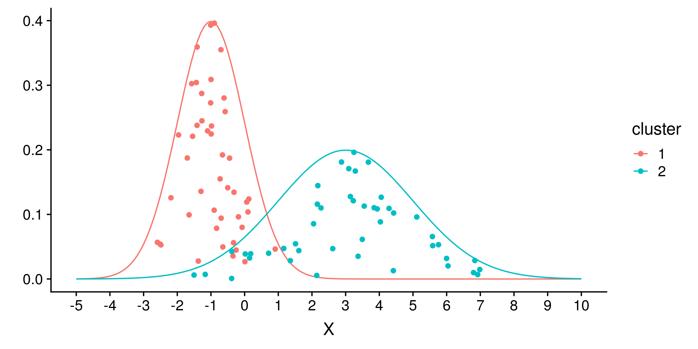
We can estimate the means m₁ and m₂ of the two clusters, under the true model of two gaussian clusters of standard deviation 1 and 2. Under this true model, the likelihood of a sample x is the sum of the probability densities of x for the normal distributions N(m₁, 1) and N(m₂, 2).

We can use a uniform prior of -10 to 10 for both means, which excludes any probability that either mean is outside that range. The unnormalized posterior density is the product of all likelihoods and priors. Usually we work in log space because such a product will often exceed the precision of floating point numbers, and so take the sum of log likelihoods and log priors as the log probability density.

Using the Python code (at the end of this post), I ran an MCMC “chain” for 100,000 iterations, sampling every 100th iteration, for a total of 1000 state samples:

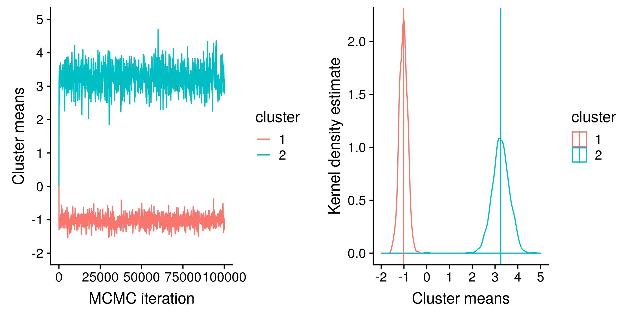
On the left hand side, the “traces” of m₁ (red) and m₂ (blue) estimates are shown. These traces track the value of m₁ and m₂ at each sampled iteration of the MCMC chain. The “hairy caterpillar” appearence of both traces suggests (but do not guarantee) that we have a good sample of the posterior distribution.

On the right hand side, KDE is used to estimate the posterior distribution of m₁ and m₂ from the same MCMC sample values. The mean of a posterior sample, shown as vertical lines, is an estimate of the expectation of the posterior distribution, and in this case the estimates are close to the true values of -1 and 3. The standard deviation of the posterior distribution is commonly known as the standard error.

But what happens if the posterior distribution is not smooth? One way this can happen is if the model used for estimating parameter values is very different from the true generative process. Needless to say, this is a common situation in biological sequence analysis.

Let’s change the generative model to three 1-dimensional gaussian clusters of means -1, 1 and 3, and each with a standard deviation of 1. Drawing 30 samples from each cluster:

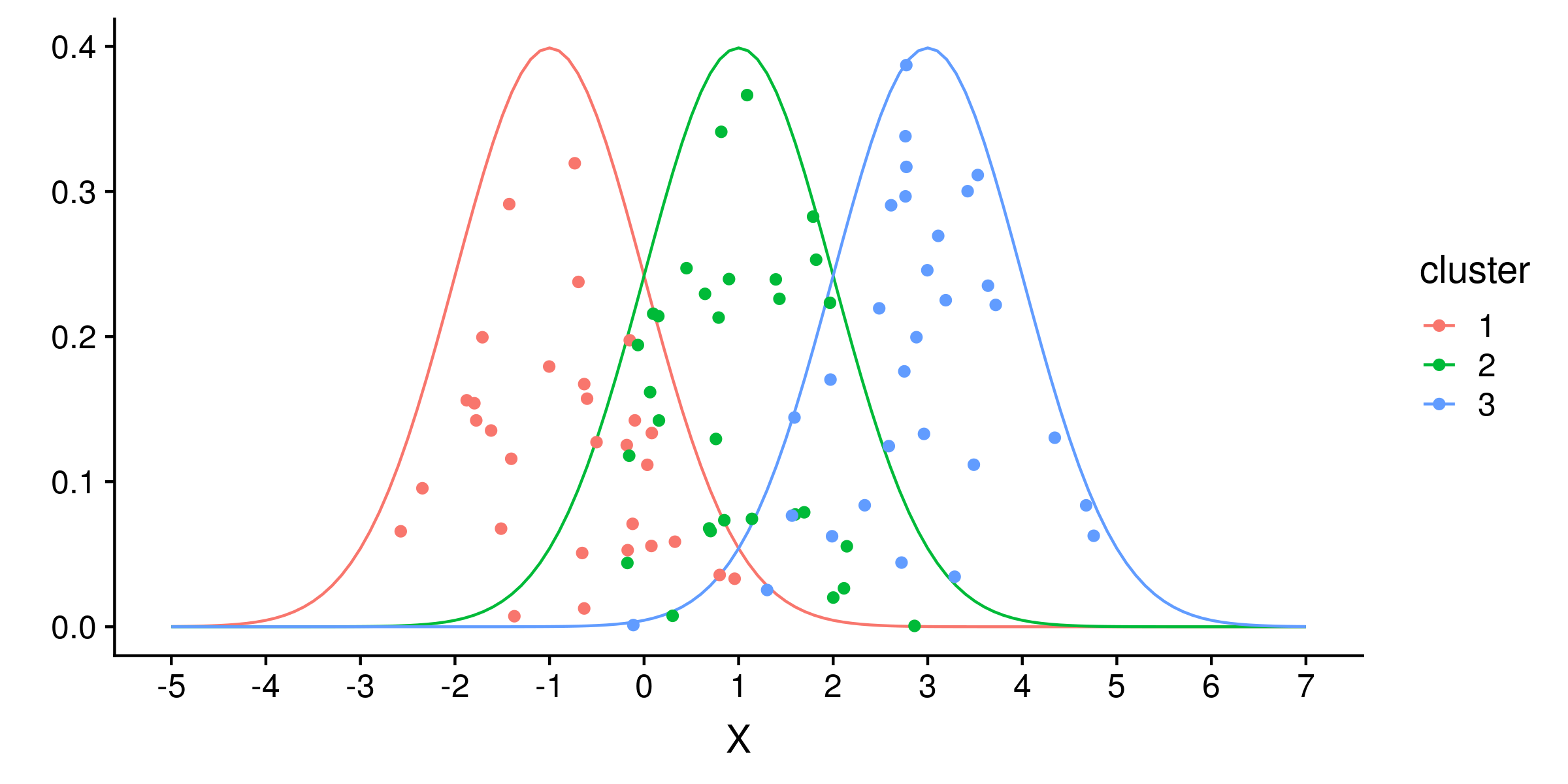
And running the now incorrect model based on two clusters of different standard deviations:

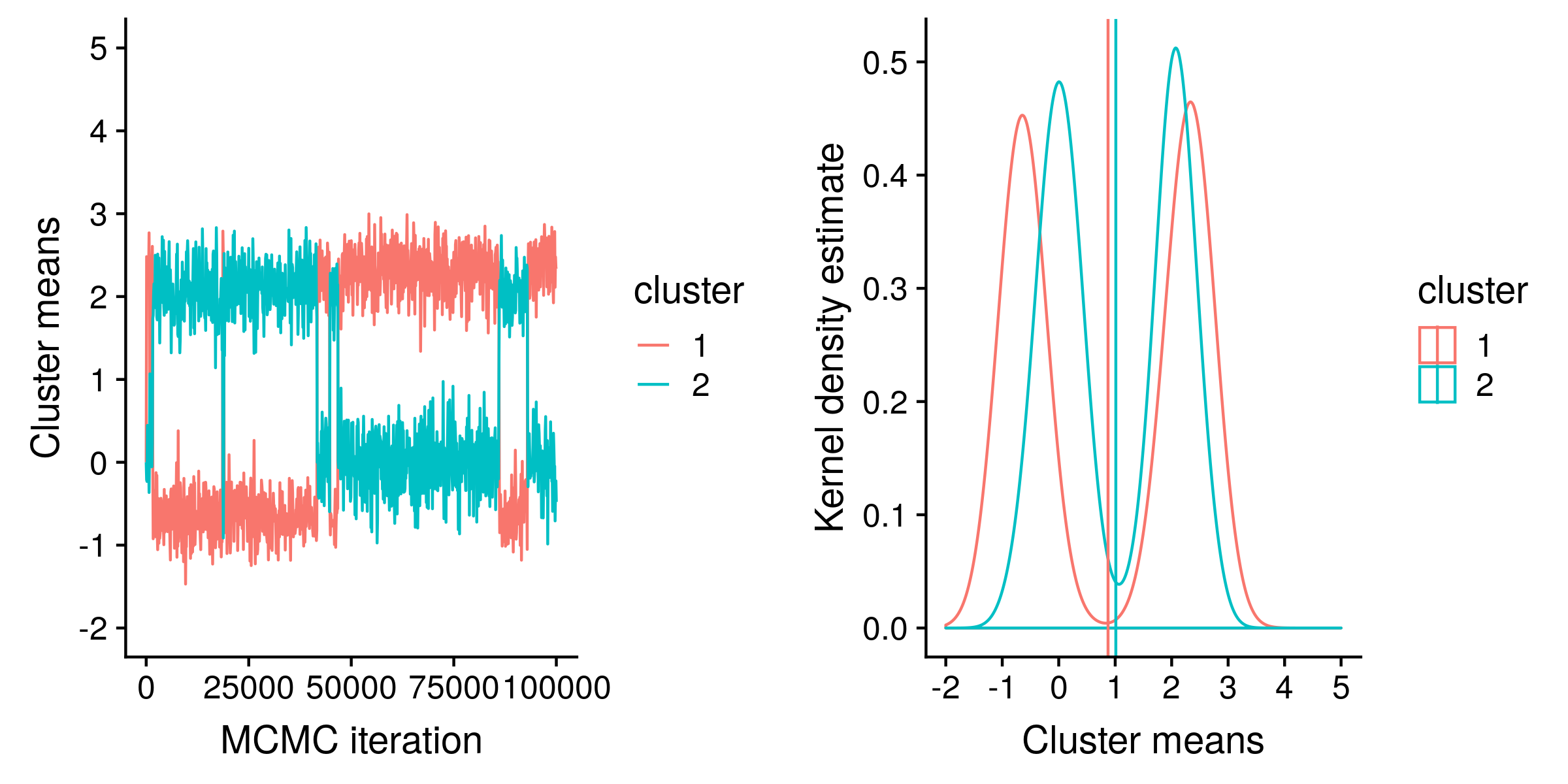
From the traces and from the density plot you can see that the posterior distribution is bimodal. One mode is where the first cluster in our model (with a standard deviation of 1) is centered on the first true cluster (with a mean of -1), and the second cluster in our model (with a standard deviation of 2) is centered between the second and third true clusters (with means of 1 and 3). The other mode is where the first model cluster is centered on the last true cluster, and the second model cluster is “shared” between the first and second true clusters.

Because our model is so wrong, the posterior expectations are now unreliable. A naïve interpretation of the expectations is that there are two gaussian clusters both centered on 1, which would be quite incorrect.

From the trace plot, you can see that the frequency of switching between the modes is very low, and we no longer have two hairy caterpillars, which means the posterior sample is not yet representative of the true posterior distribution.

To get a representative sample, either we could run our MCMC for many (many) more iterations, and then there will be enough switching between the modes for our plot to resemble two overlapping hairy caterpillars. Then the estimate of the posterior distribution, e.g. the estimates of cluster mean expectations, will be accurate. Of course the posterior distribution and expectations themselves are not accurate because of the wrong model.

Hastings relaxed the MCMC algorithm to work with asymmetric proposal distributions. There are also many techniques to improve the performance of MCMC, for example parallel tempering. Code for the MCMC algorithm used for these examples is below:

import csv
import numpy
import scipy.stats as stats

n_per_cluster     = 45     # number of samples per cluster
n_mcmc_iterations = 100000 # run the MCMC chain for 100,000 iterations
sample_frequency  = 100    # record every 100th iteration as a sample

# generate random samples from the two clusters
c1_data = numpy.random.standard_normal(n_per_cluster) - 1     # cluster 1, mean = -1, sd = 1
c2_data = numpy.random.standard_normal(n_per_cluster) * 2 + 3 # cluster 2, mean =  3, sd = 2

data = numpy.concatenate([c1_data, c2_data])

c1_mean = 0.0 # the initial value of the mean of cluster 1
c1_sd = 1.0   # the fixed value of the standard deviation of cluster 1

c2_mean = 0.0 # the initial value of the mean of cluster 2
c2_sd = 2.0   # the fixed value of the standard deviation of cluster 2

# specify a uniform prior from -10 to 10
uniform_prior_lower = -10.0
uniform_prior_width = 20.0

likelihoods = stats.norm.pdf(data, c1_mean, c1_sd) + stats.norm.pdf(data, c2_mean, c2_sd)
c1_mean_prior = stats.uniform.pdf(c1_mean, uniform_prior_lower, uniform_prior_width)
c2_mean_prior = stats.uniform.pdf(c2_mean, uniform_prior_lower, uniform_prior_width)
log_posterior = numpy.sum(numpy.log(likelihoods)) + numpy.log(c1_mean_prior) + numpy.log(c2_mean_prior)

# set up the file to output MCMC sample states
output_filename = "mcmc_01.csv"
output_file = open(output_filename, "w")
output_writer = csv.writer(output_file)

# write a header to the output file
output_header = ["sample", "log_posterior", "c1_mean", "c2_mean"]
output_writer.writerow(output_header)

# for each iteration in the MCMC chain
for i in range(n_mcmc_iterations):
	# record the current state once out of every "sample_frequency" iterations
	if (i % sample_frequency) == 0:
		output_row = [i, log_posterior, c1_mean, c2_mean]
		output_writer.writerow(output_row)

	# The proposed change (delta) made to the mean parameter is chosen from a
	# uniform distribution between -0.5 and 0.5.
	proposal_delta = numpy.random.random_sample() - 0.5

	if numpy.random.random_sample() < 0.5: # change c1 half of the time
		proposed_c1_mean = c1_mean + proposal_delta
		proposed_c2_mean = c2_mean
	else: # change c2 the other half
		proposed_c1_mean = c1_mean
		proposed_c2_mean = c2_mean + proposal_delta

	# recalculate likelihoods and priors based on the proposed c1 and c2 means
	proposed_likelihoods = stats.norm.pdf(data, proposed_c1_mean, c1_sd) + stats.norm.pdf(data, proposed_c2_mean, c2_sd)
	proposed_c1_mean_prior = stats.uniform.pdf(proposed_c1_mean, uniform_prior_lower, uniform_prior_width)
	proposed_c2_mean_prior = stats.uniform.pdf(proposed_c2_mean, uniform_prior_lower, uniform_prior_width)

	# calculate the log unnormalized posterior density, and from that the acceptance ratio
	proposed_log_posterior = numpy.sum(numpy.log(proposed_likelihoods)) + numpy.log(proposed_c1_mean_prior) + numpy.log(proposed_c2_mean_prior)
	log_acceptance_ratio = proposed_log_posterior - log_posterior
	acceptance_ratio = numpy.exp(log_acceptance_ratio)

	# if the acceptance ratio is greater than 1, always accept the proposed c1 or c2 mean
	# if it less than 1, accept in proportion to the acceptance ratio
	if numpy.random.random_sample() < acceptance_ratio:
		c1_mean = proposed_c1_mean
		c2_mean = proposed_c2_mean

		log_posterior = proposed_log_posterior

# write the final state to the output file
output_row = [n_mcmc_iterations, log_posterior, c1_mean, c2_mean]
output_writer.writerow(output_row)

For a more detailed description of Bayesian theory, read chapter 6 of Ziheng Yang’s Molecular Evolution. For a more detailed description of MCMC, read chapter 7 of Yang’s book. For an in-depth introduction to Bayesian statistics, inference algorithms and methods, I highly recommend the excellent Puppy Book. This is also (more properly) known as Doing Bayesian Data Analysis, by John Kruschke.