Expected values of score matrices

There are many ways to compute score matrices for amino acid alignment. Typically score matrices are based on the log-odds of amino acid replacements, and so higher scores represent replacements which are more likely, and lower scores replacements which are less likely. The simplest meaningful matrix is for binary data of zeros and ones. Let’s generate a score matrix from this a priori alignment of two homologous binary sequences, which has a total length of 60 sites:

X = 010000011100011100010111101011000110111110001110010000100010
Y = 000100011101011110111000111001101110101000111010110010110100

We will refer to indices of the X sequence as i, and indices of the Y sequence as j. There are four possible site patterns in this alignment; 00, 11, 01 and 10. Count up the number of occurances of each site patten in the a priori alignment, and use them to fill in a count matrix:

	0	1
0	18	10
1	14	18

Now convert the counts to probabilities. For the diagonal probabilities P₁₁ and P₀₀, simply divide the count by the total length in sites. For the other probabilities, let’s assume that our molecular evolutionary process is time-reversible, so that the probability P_ij equals P_ji. Therefore divide the average of P₀₁ and P₁₀ by the total length in sites:

	0	1
0	0.3	0.2
1	0.2	0.3

To compute a log-odds score matrix we also need the expected probabilities for non-homologous sequences. This is simply the product of the base frequencies q_i and q_j. Again making the assumption that our process is time-reversible, we will take the average of the base frequencies in the X and in the Y sequences: in our example this equals 0.5 for the binary character 0 and 0.5 for the binary character 1. The matrix of expected probabilities is therefore:

	0	1
0	0.25	0.25
1	0.25	0.25

The formula to compute log-odds scores in half-bit units is 2log₂(P_ij/q_iq_j). The scores in half-bits are therefore:

	0	1
0	0.53	-0.64
1	-0.64	0.53

To improve computational performance, the resulting scores are usually rounded to the nearest integer. Our final score matrix becomes:

	0	1
0	1	-1
1	-1	1

If we score a gapless alignment of two non-homologous sequences using this score matrix, since our base frequencies are equal, any of the four nucleotide pairs (00, 11, 01 and 10) are equally likely. The score S_ij will be -1 or 1 with equal probability, so the expected value E(S) of aligning two non-homologous characters is zero:

E(S) = q₀q₀ × S₀₀ + q₁q₁ × S₁₁ + q₀q₁ × S₀₁ + q₁q₀ × S₁₀ = 0.25 + 0.25 - 0.25 - 0.25 = 0

Non-negative expected values have undesirable consequences for local alignment. To illustrate this, I simulated 20 gapless alignments of random, non-homologous sequences of 500 sites each and computed their gapless local alignment scores (where negative scores are reset to zero) along the diagonal beginning at (0, 0) for three different score matrices:

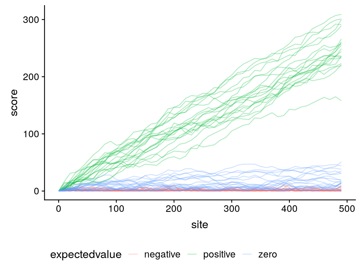
In blue is our score matrix where matches have a log-odds score of 1 and mismatches -1, and the expected value for non-homologous gapless alignments is zero. In red, the score of matches is 1 and mismatches -2, making the expected value negative. In green, matches are 2 and mismatches -1, making the expected value positive.

From this simulation it can be seen that when local alignment algorithms like Smith–Waterman are used with the non-negative expected value score matrices, very long local alignments can be returned of entirely non-homologous sequences.

To avoid this, local alignment should therefore be used with score matrices where the expected value for non-homologous sequence alignments is negative. For more information about the trouble with non-negative expected score values, see chapter 2 of Biological sequence analysis by Durbin et al.