Smith–Waterman

The Smith–Waterman algorithm is basically the Needleman–Wunsch, but with a few modifications to turn it into a local alignment algorithm. These are:

1. Whenever the alignment score for a pair of sites/residues and or a site/residue and a gap is negative, reset the score to zero.
2. Do not draw outgoing arrows from F-matrix cells with zero scores.
3. To generate the local alignment with the maximum score, start from the F-matrix cell with the highest score
4. Proceed as per Needleman–Wunsch, stopping when a cell with a zero score is reached.

To demonstrate the algorithm, let’s align the first ten residues of CLV1 X=MAMRLLKTHL with the first eight residues of SUNN Y=MKNITCYL based on the BLOSUM50 matrix and a linear gap penalty of -8 (this is the same toy example we used for Needleman–Wunsch.

Fill in a zero in the top left corner, but this time fill in the first row and column with all zeros, as we do not permit negative values in the Smith–Waterman F-matrix:

In the first empty cell, consider aligning the X residue with a gap (left arrow), the Y residue with a gap (up arrow), or aligning both X and Y residues (diagonal arrow). The possible scores are -8, -8 or 7 respectively. Since 7 is the highest, fill in seven and draw a diagonal arrow.

In the next cell, aligning the X residue with a gap (left arrow) will result in a score of 0 + -8 = -8, and aligning the Y residue with a gap will result in a score of 7 + -8 = -1. Matching the X and Y residues M and A will result in a score of 0 + -1 = -1. Since none of these scores are at least zero, fill in a zero. Since the final score is zero, do not draw any outgoing arrows.

Fill in the rest of the F-matrix using the same rules:

Now identify the highest scoring value in the entire matrix. This happens to be the bottom right hand cell, which has a score of 13. This is the alignment score of the best possible local alignment. Follow the arrows until a zero scoring cell is encountered:

Along this highest scoring path, we have eight diagonal arrows in a row, so in this example simply align the final eight residues from both X and Y sequences:

MRLLKTHL
MKNITCYL

Notice that unlike in the global alignment example, the first two residuesof the X sequence (M and A) are not aligned to anything and not present in the final local alignment.

A more realistic illustration of the difference between the global and local alignments is shown by comparing the homologous receptor proteins CLV1 and CLV2, which unlike CLV1 and SUNN are not homologous across their entire lengths.

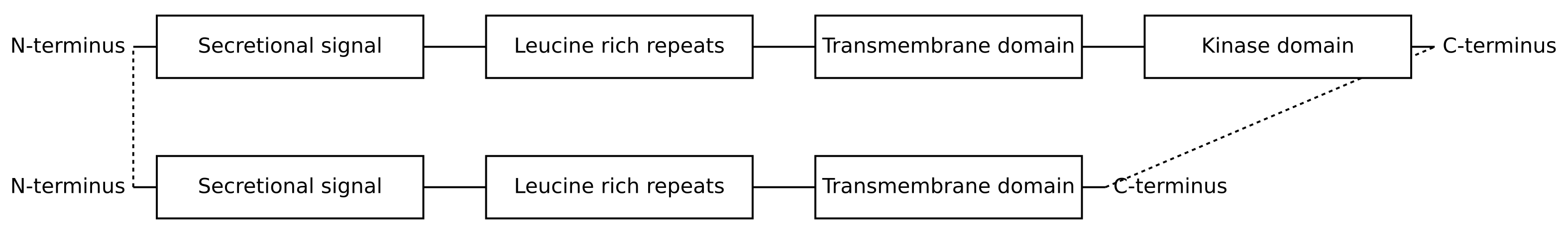
CLV1 and CLV2 both contain a secretion signal towards their N-terminus (which directs the cell to export the protein), a series of leucine rich repeats (which bind to plant hormones or epitopes), and a transmembrane domain (which anchors the protein to the cell membrane). However when CLV1 and CLV2 split through a duplication of the ancestral protein, CLV2 lost its kinase domain (which transmits a signal to the interior of the cell).

Global alignment is based on the assumption that the proteins being aligned are homologous across basically their entire length. So despite the fact that CLV2 is missing an entire domain at its N-terminus, Needleman–Wunsch will try to align the entire length of CLV2 to the entire length of CLV1:

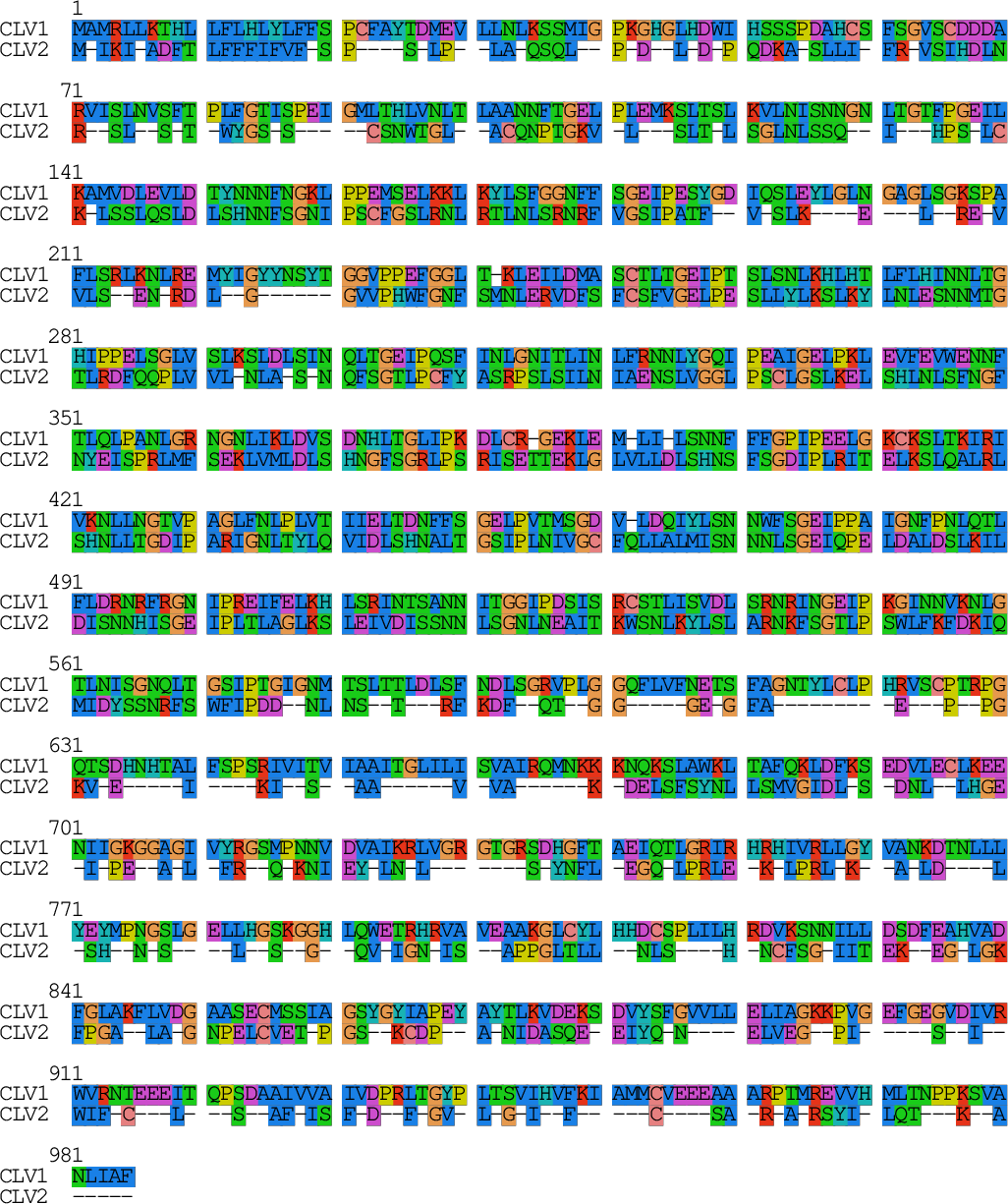
You can see the effect this has on the pairwise alignment, where many CLV2 residues are aligned to the kinase domain of CLV1 (from around position 701):

It is clearly inappropriate to use global alignment in this case, where every residue of both proteins is aligned (either with a residue from the alternate protein or with a gap). Instead we should use local alignment.

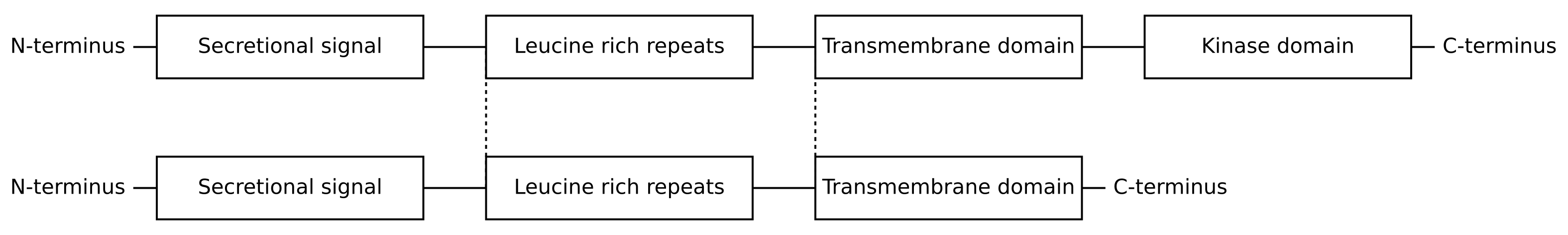
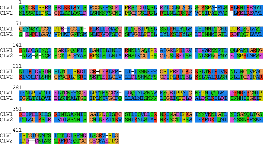
For each local alignment, only a particular region from each protein will be aligned. In the case of CLV1 and CLV2, the region with the highest local alignment score is from the start of the leucine rich repeats through to the beginning of the transmembrane domain:

Looking at the local alignment for this region generated using the Smith–Waterman algorithm, we can see that most residues are alignable and that these regions are identifiably homologous despite hundreds of millions of years of evolutionary divergence:

For more information about Smith–Waterman, see chapter 2 of Biological sequence analysis by Durbin et al., and Wikipedia.

Update 13 October 2019: for an another perspective on sequence alignment, including local alignment, consult Chapter 5 of Bioinformatics Algorithms (2nd or 3rd Edition) by Compeau and Pevzner.