Pseudocounts

When computing PSSMs, averaging does not take into account the amount of information available in a multiple sequence alignment (MSA) used to construct a PSSM. Even when the aligment includes many sequences, averaging will still flatten the distribution of scores, unnecessarily reducing the power of the PSSM.

Pseudocount methods elegantly allow the data to mostly determine PSSM scores when the MSA is large in the number of sequences, while still avoiding the problem of noisy PSSMs with negative infinity scores when the number of sequences is few. Psuedocount methods are actually a kind of Bayesian inference, a statistical framework and philosophy where parameter estimates are informed more by a “prior” distribution when the quantity of data is small, and more informed by the data when the quantity of data is large. To demonstrate why and how pseudocount methods are Bayesian¹, let’s start with the simple example of “red” and “green” alleles.

To calculate the likelihood, we need to specify some kind of model which we assume generated the data. A simple model for PSSMs with two alleles is the Bernoulli process. In this model, the probability of observing a red allele is P, and the probability of observing a green allele is 1 - P. Each observation is assumed to be independent, in other words there is no correlation between sequences beyond the value of P. For this example we will estimate P separately, hereafter called θ, for each column in the MSA, and assume each value of θ is independent. In other words the allele distribution of one column has no effect on any other column.

Under our model, the likelihood of any site i in any sequence is θ_i when the allele at that site is red, and 1 - θ_i when it is green. The product of likelihoods of site i for all sequences is the likelihood of column i, and the likelihood of the entire PSSM is the product of all column likelihoods.

Consider the following multiple sequence alignment of just two sequences, three columns each, and only red or green alleles:

RRG
RGG

To calculate the likelihood distribution over θ for each column, I calculated the likelihood for 100 evenly spaced values of theta between 0 and 1. This is known as a grid search, and the result looks like this:

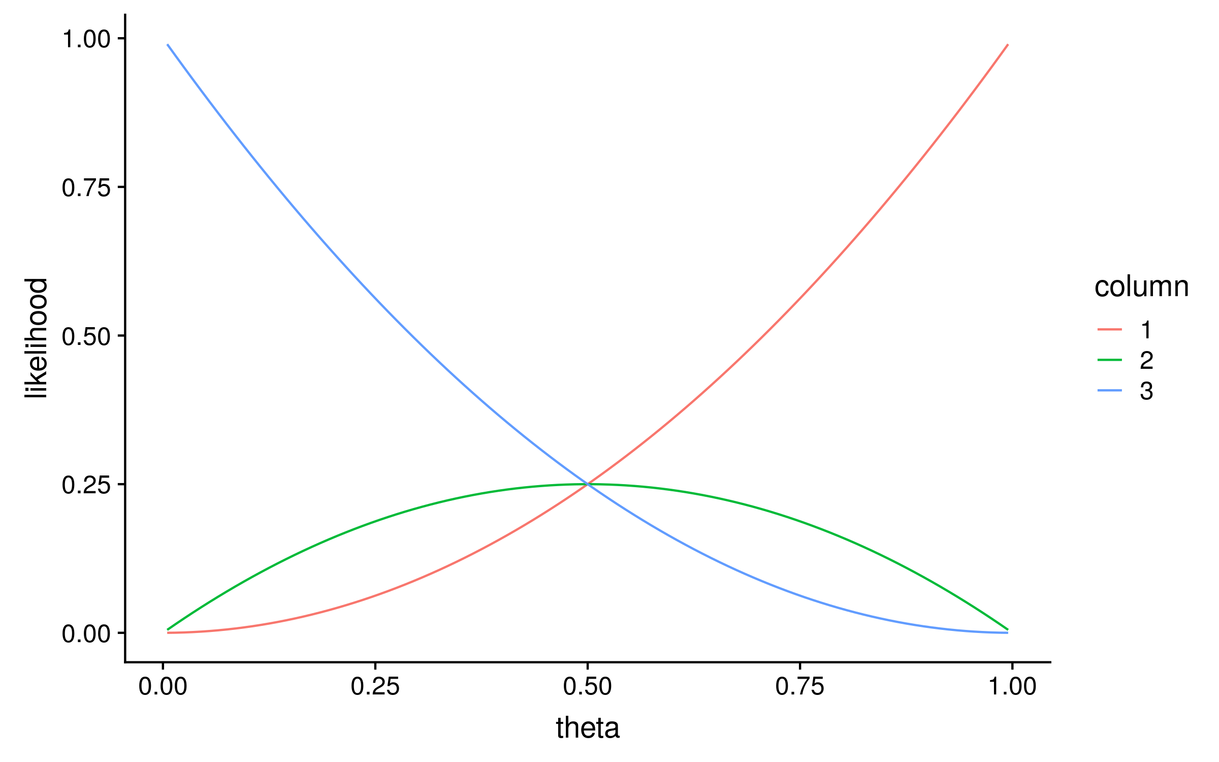
Notice that the maximum likelihood values correspond exactly to the proportion of red alleles in the original multiple sequence alignment; 1, 0.5 and 0. We can therefore describe the original method for computing PSSMs as a maximum likelihood method!

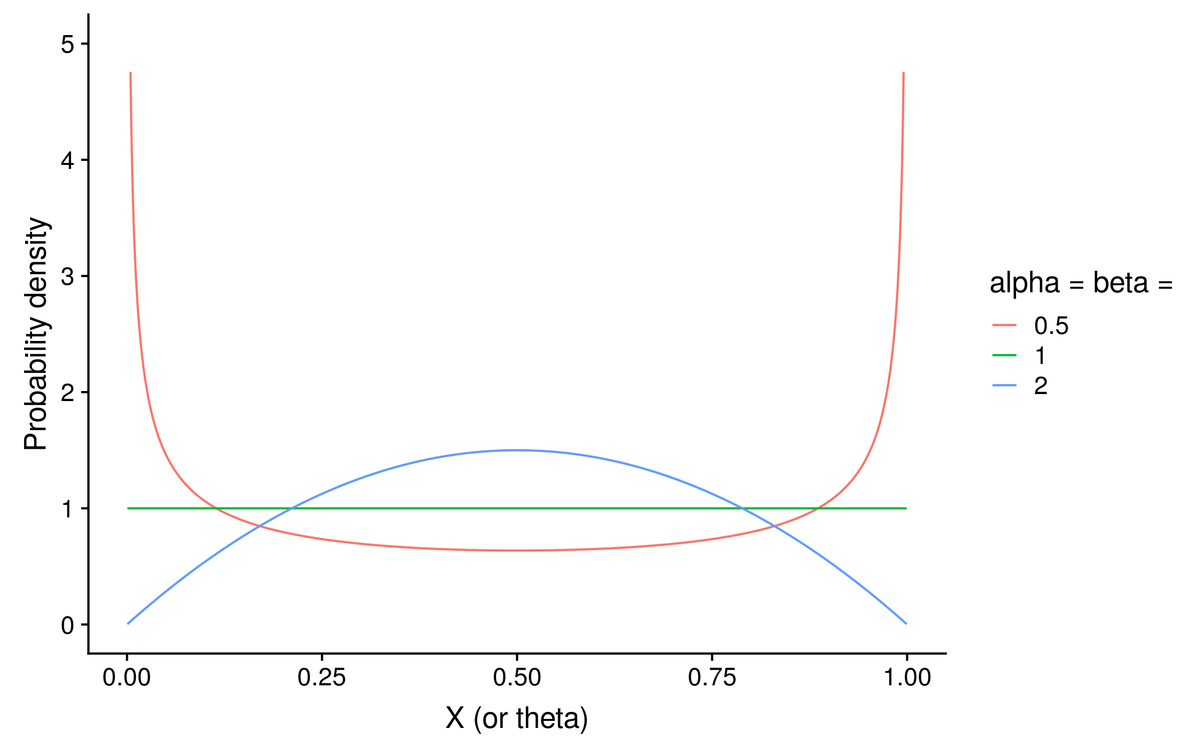
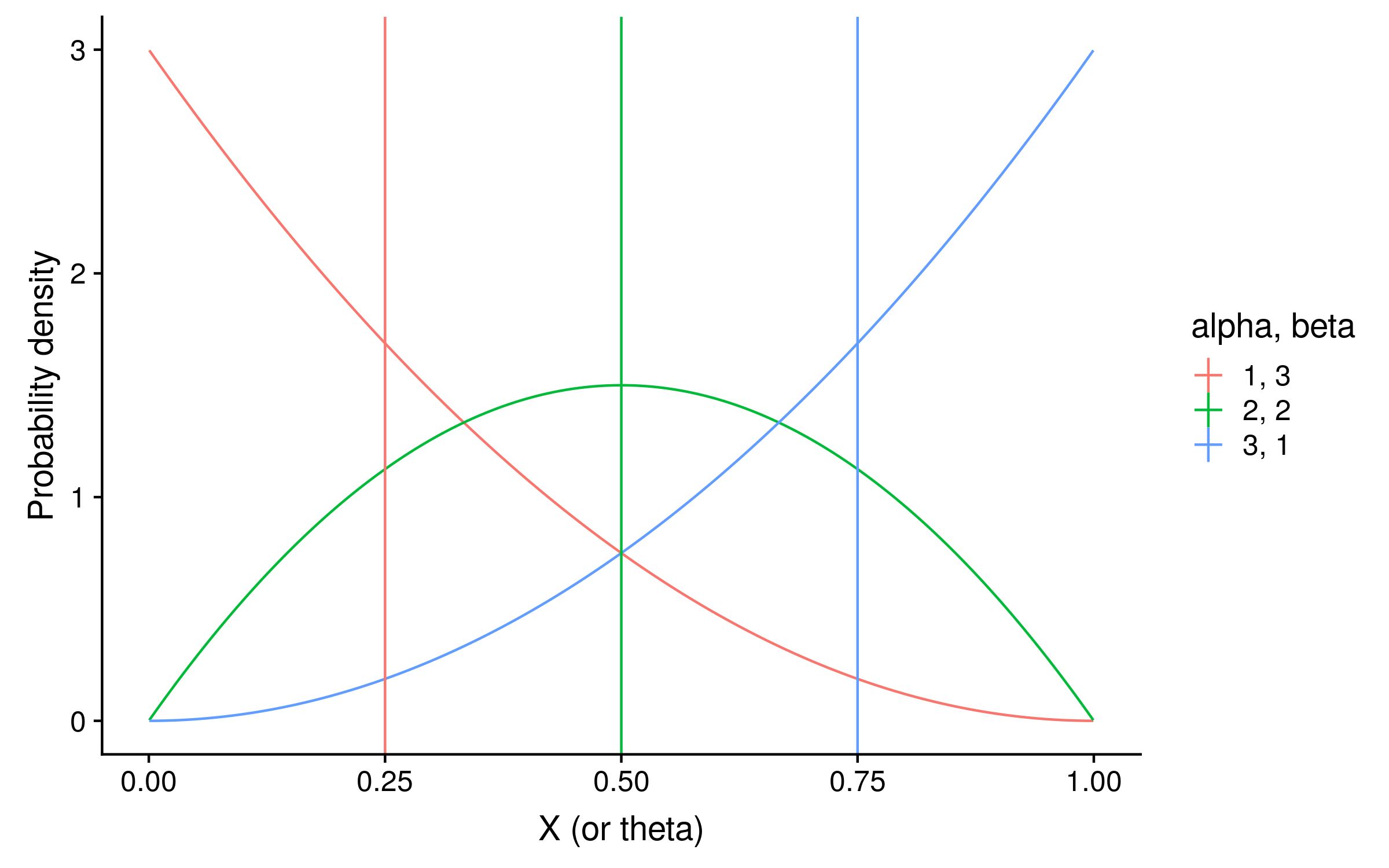
Since this is Bayesian inference, we also need a prior. With just two alleles, we can use a beta distribution as the prior on θ. Beta distributions take two parameters, alpha and beta. If alpha = beta, then the distribution is symmetric. For a PSSM prior distribution, setting alpha = beta < 1 means that we expect θ to be closer to 0 or 1 for a given column. Setting alpha = beta > 1 means that we expect θ to be closer to 0.5 at each column. Setting alpha = beta = 1 is the same as a uniform prior, and means we have no opinion what the distribution of θ.²

The shape of the beta distribution when alpha = beta < 1 (red) shows how in that case the probability is concentrated around 0 and 1, whereas when alpha = beta > 1 the probability is concentrated around 0.5:

Although calculating the posterior distribution directly is often intractable because of the tricky marginal likelihood, in this 1-dimensional case bounded by 0 and 1, we can calculate an unnormalized posterior distribution from the likelihood and prior alone by using a grid search.

If the prior is a beta distribution B(alpha = beta = 1), the prior density will be 1 for every value of θ, and the unnormalized posterior distribution will be identical to the likelihood distribution. For our Bayesian PSSMs, we can use the expected values of θ as the probabilities of observing a red allele. The expected values are just the mean of the posterior distribution of theta values.³ Here I have plotted the expectations as vertical lines:

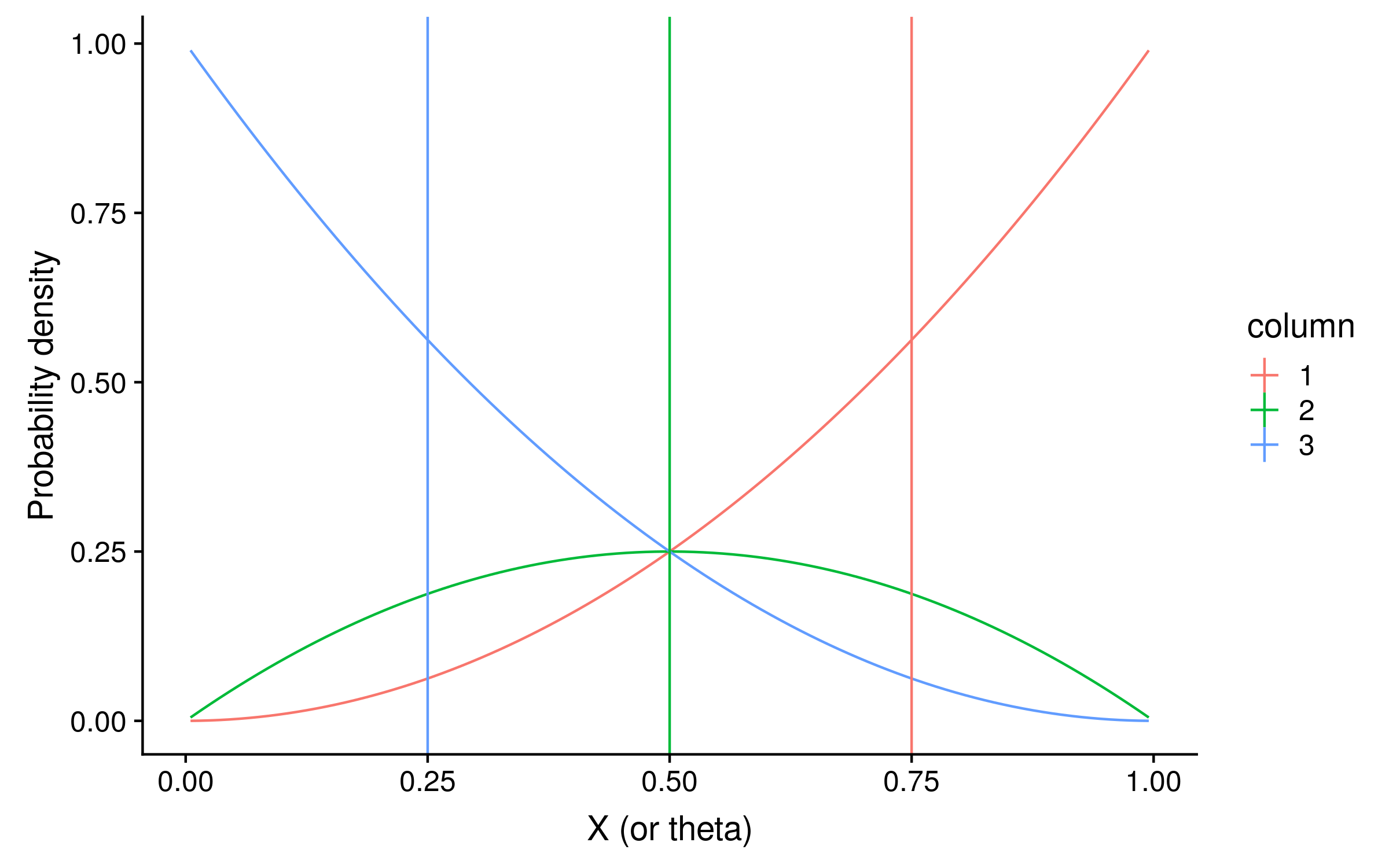
The expectations are 0.75, 0.5 and 0.25 for columns 1, 2 and 3 respectively. You might notice that these are suspiciously round numbers… and they are.

While this grid search is easy enough for two alleles, consider amino acids. In that case θ is now a vector of 19 values for each column (although there are 20 amino acid, the probability of the 20th must be 1 minus the sum of theta, so that the total probability sums to 1). A grid search of the same precision would therefore require 100¹⁹ = 10³⁸ likelihood calculations for each column. How big is that number? It is this big:

100,000,000,000,000,000,000,000,000,000,000,000,000

Clearly we need a faster method, at least for protein sequences. Fortunately the beta distribution is the conjugate prior for the Bernoulli process! Consider the following scenario:

Given:

1. The prior distribution is a Gaussian distribution
2. The likelihood model is a Gaussian process

Then, because the product of two Gaussians is a Gaussian,

1. The posterior distribution will be a Gaussian distribution

When the prior and posterior distributions are the same kind of parametric distribution given the likelihood model, we call this parametric distribution a conjugate prior. Since Bayesian inference can be thought of as updating the prior distribution to arrive at the posterior distribution, when using a Gaussian conjugate prior we can simply update the mean and standard deviation to arrive at the posterior.

Luckily for us, the beta distribution is a conjugate prior for the Bernoulli process! That is:

Given:

1. The prior distribution is a beta distribution
2. The likelihood model is a Bernoulli process

Then,

1. The posterior distribution will be a beta distribution

Updating the alpha and beta parameters of the beta distribution is remarkably easy. Parameters of prior distributions are known as hyperparameters, and in our example the posterior value of alpha for a given column is simply the sum of red alleles in the column, plus the alpha hyperparameter. The posterior value of beta is simply the number of green alleles in the column, plus the beta hyperparameter. For each column in our example, using a uniform prior of B(alpha = 1, beta = 1), the posterior alpha and beta parameters are:

1. alpha = 2 + 1 = 3, beta = 0 + 1 = 1
2. alpha = 1 + 1 = 2, beta = 1 + 1 = 2
3. alpha = 0 + 1 = 1, beta = 2 + 1 = 3

These distributions with their expectations look like the following:

They are exactly the same shape as the grid search distribution. However unlike the grid search they are normalized so that the integral over θ sums to 1, which makes the column 2 beta distribution look taller.

To calculate the expectation, we can use the mean of each beta distribution, which is alpha / (alpha + beta). In our example the expectations are 3 / 4 = 0.75, 2 / 4 = 0.5, and 1 / 4 = 0.25. Notice that these posterior expectations of red allele frequency are the same as calculating the observed probability of red alleles, except before calculating the probability the alpha hyperparameter value is added as a pseudocount to the red allele counts, and the beta hyperparameter value is added as a pseudocount to the green allele counts.

To sum all the above up in a single sentence: adding a pseudocount of 1 to each allele in each column when calculating the allele frequencies is identical to Bayesian inference of the allele frequencies with a uniform prior!

It’s straightforward to see how pseudocounts have less effect as the amount of data increases. In an example with 1000 sequences where there were 1000 red alleles in the first column, the Bayesian estimates of the frequency of red and green alleles is 1001 / 1002 and 1 / 1002, or approximately 0.999 and 0.001 respectively.

For sequences with more than two alleles (e.g. nucleotides with four, amino acids with 19), instead of a Bernoulli process (which only has two outcomes), the likelihood model is a multinomial process. Instead of a beta distribution, the conjugate prior is a Dirichlet distribution. This is the multinomial generalization of the beta distribution, and replaces the single alpha and beta parameters with a vector of alpha parameters.

For a uniform (or flat) Dirichlet distribution, all alpha values are 1, and we can still just add 1 to each count before calculating the allele probabilities in that case.

To learn more about pseudocounts, read Henikoff and Henikoff on PSSMs. For a brief introduction to conjugate priors, check out section 6.3.2 of Ziheng Yang’s Molecular Evolution. For a more detailed treatment of beta and Dirichlet conjugate priors, read Michael I. Jordan’s The Exponential Family: Conjugate Priors.

Update 13 October 2019: for another perspective on applying pseudocounts to PSSMs, consult the “Laplace’s Rule of Succession” section of Chapter 2 of Bioinformatics Algorithms (2nd or 3rd Edition) by Compeau and Pevzner.

1. Bayesian inference is not universally popular and I wonder if the term “pseudocounts” was coined to sell the method as a pragmatic way to adjust PSSM scores, rather than a Bayesian method. But that’s just a guess ¯\_(ツ)_/¯ ↩

2. This is an oversimplification, see section 6.3.2 of Molecular Evolution for alternative “noninformative” beta priors ↩

3. It doesn’t matter that the posterior distribution is unnormalized, since normalization won’t affect the mean of theta ↩