Hill climbing and NNI

The Sankoff algorithm can efficiently calculate the parsimony score of a tree topology. Felsenstein’s pruning algorithm can efficiently calculate the probability of a multiple sequence alignment given a tree with branch lengths and a substitution model. But how can the tree with the lowest parsimony score, or highest likelihood, or highest posterior probability be identified?

Possibly the simplest algorithm that can do this for most kinds of inference is hill-climbing. This algorithm basically works like this for maximum likelihood inference:

1. Initialize the parameters \(\theta\)
2. Calculate the likelihood \(L = P(D\vert\theta)\)
3. Propose a small modification to \(\theta\) and call it \(\theta'\)
4. Calculate the likelihood \(L' = P(D\vert\theta')\)
5. If \(L' > L\), accept \(\theta \leftarrow \theta'\) and \(L \leftarrow L'\)
6. If stopping criteria are not met, go to 3

You may notice that without stopping criteria, the algorithm is an infinite loop. How do we know when to give up? Three obvious criteria that can be used are:

1. Stop after a certain number of proposals are rejected in a row (without being interrupted by any successful proposals)
2. Stop after running the algorithm for a certain length of time
3. Stop after running the algorithm for a certain number of iterations through the loop

For maximum a posteriori inference, we also need to calculate the prior probability \(P(\theta)\). Because the marginal likelihood \(P(D)\) does not change, following Bayes’ rule the posterior probability \(P(\theta\vert D)\) is proportional to \(P(D\vert\theta)P(\theta)\), which we might call the unnormalized posterior probability. So instead of maximizing the likelihood, we instead maximize the product of the likelihood and prior, which we have to recalculate for each proposal. The algorithm becomes:

1. Initialize the parameters \(\theta\)
2. Calculate the unnormalized posterior probability \(P = P(D\vert\theta)P(\theta)\)
3. Propose a small modification to \(\theta\) and call it \(\theta'\)
4. Calculate the unnormalized posterior probability \(P' = P(D\vert\theta')P(\theta')\)
5. If \(P' > P\), accept \(\theta \leftarrow \theta'\) and \(P \leftarrow P'\)
6. If stopping criteria are not met, go to 3

For maximum parsimony inference, we simply need to calculate the parsimony score of our parameters, so I will describe this as a function \(f(D,\theta)\) which returns the parsimony score. The algorithm becomes:

1. Initialize the parameters \(\theta\)
2. Calculate the parsimony score \(S = f(D,\theta)\)
3. Propose a small modification to \(\theta\) and call it \(\theta'\)
4. Calculate the parsimony score \(S' = f(D,\theta')\)
5. If \(S' < S\), accept \(\theta \leftarrow \theta'\) and \(S \leftarrow S'\)
6. If stopping criteria are not met, go to 3

Note that the inequality is reversed in step 5 for maximum parsimony. These are all described for general cases, but for phylogenetic inference $\theta$ will correspond to a tree topology, and possibly branch lengths (for non-ultrametric trees) or node heights (for ultrametric trees). Maximum parsimony is unaffected by branch lengths, so $\theta$ is only the tree topology. Proposing changes to branch lengths or node heights is relatively simple because we can use some kind of uniform, Gaussian or other proposal distribution. But how do we propose a small change to the tree topology?

A huge amount of research has gone into tree changing “operators,” but the simplest and most straightforward is nearest-neighbor interchange, or NNI. This works by isolating an internal branch of a tree, which for an unrooted tree always has four connected branches. The four nodes at the end of the connected branches may be tips or other internal nodes, because NNI can work on trees of any size.

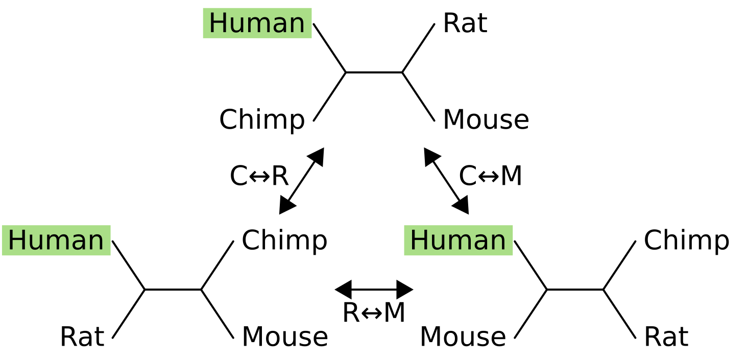
One of the nodes is fixed in place (in this example, humans), and its sister node is exchanged with one of the two other nodes.

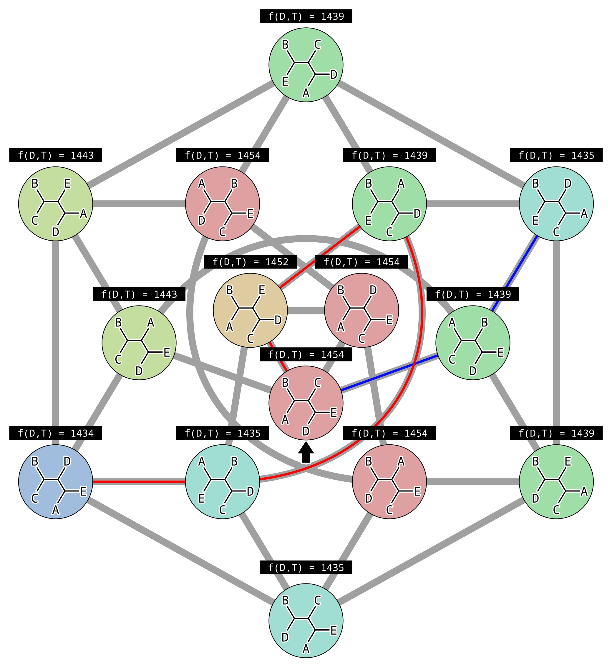
For example the NNI move from the tree at the top to the tree in the bottom-right exchanges mouse (M) with chimpanzee (C), causing the sister of humans to change from chimps to mice. For four taxon trees there are only three topologies, and they are all connected by a single NNI move. For five taxon unrooted trees there are fifteen topologies and not all are connected:

In the above example, each gray line represents an NNI move between topologies, and there is (made-up) parsimony scores above each topology. There are two peaks in parsimony score, one for the tree (((A,E),D),(B,C)) where the parsimony score is 1434, and one for the tree (((B,E),D),(A,C)) where the parsimony score is 1435. Since the second peak has a higher parsimony score, it is a local and not the global optimal solution.

This illustrates the biggest problem with hill climbing. Because we only accept changes that improve the score, once we reach a peak where all connected points in parameter space (unrooted topologies in this case) are worse, then we can never climb down. Imagine we initialized our hill climbing using the topology indicated by the black arrow. By chance we could have followed the red path to the globally optimal solution… or the blue path to a local optimum.

One straightforward way to address this weak point is to run hill climbing multiple times. The likelihood, unnormalized posterior probability or parsimony scores of the final accepted states for each hill climb can be compared, and the best solution out of all runs accepted, in the hope that it corresponds to the global optimum.

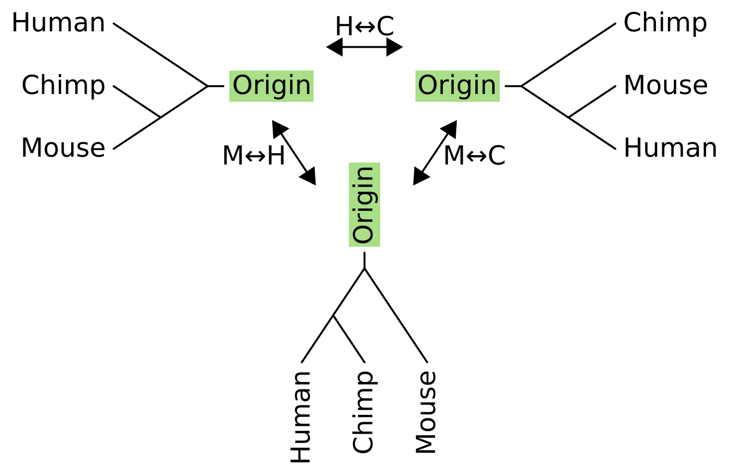
What about NNI for rooted trees? It works in a very similar way, but we have to pretend that there is an “origin” tip above the root node, and perform the operation on the unrooted equivalent of the rooted tree.

As with unrooted NNI, we can now pick any internal branch of the tree to rotate subtrees or taxa around. Connected to the head of an internal branch of a rooted tree is two child branches, and connected to the tail is a parent branch and “sister” branch. For rooted NNI, we fix the parent branch and swap its sister with one of the child branches.

For three taxon rooted trees, there is only one internal branch and the parent of this internal branch is the origin. In this example, the sister to the origin for the tree on the left is humans, so the NNI operations exchange humans with either chimps (becoming the tree on the right), or with mice (becoming the tree on the bottom).

And how do we initialize hill climbing in phylogenetics? There are a few ways.

1. Randomly generate a tree using simulation
2. Permute the taxon labels on a predefined tree
3. Use neighbor-joining if the tree is unrooted
4. Use UPGMA if the tree is rooted

The first method implies a particular model is being used to generate the tree. Models from the birth-death family or from the coalescent family are often used for this task. Another possibility is to use a beta-splitting model, see Sainudiin & Véber (2016).

The latter two methods have the advantage of starting closer to the optimal solutions, reducing the time required for a single hill climb. However when running hill climbing multiple times, the first two methods have the advantage of making the different runs more independent of each other, and therefore more likely for one to find the global optimum.