Viterbi algorithm

The Viterbi algorithm is used to efficiently infer the most probable “path” of the unobserved random variable in an HMM. In the CpG islands case, this is the most probable combination of CG-rich and CG-poor states over the length of the sequence. In the splicing case, this the most probable structure of the gene in terms of exons and introns.

Conceptually easier than Viterbi would be the brute force solution of calculating the probability for all possible paths. However the number of possible paths for two states, as in the CpG island model, is 2ⁿ where n is the number of sites. For even a short sequence of 1000 nucleotides, this equates to 2¹⁰⁰⁰ paths, or approximately 10³⁰¹. This number is about 10²²¹ times larger than the number of atoms in the observable universe.

I will first demonstrate how the algorithm works using the following simple exon-intron model:

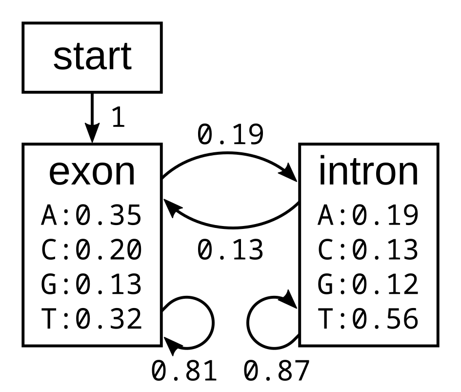
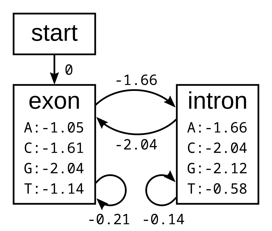
The probabilities of the model have the corresponding log-probabilities, to two decimal places:

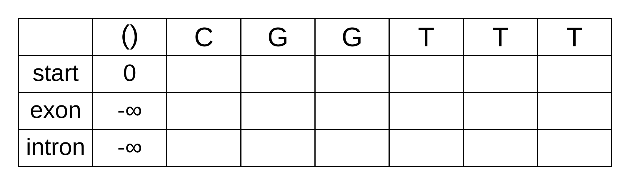
Let’s apply this simple model to the toy sequence CGGTTT.

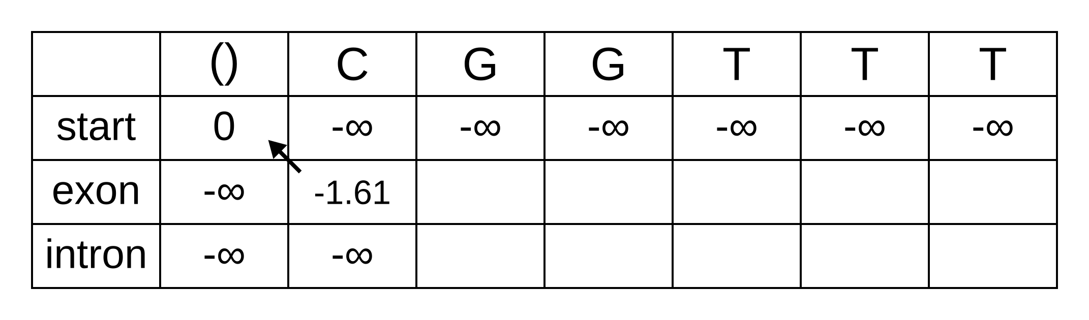
Draw up a table and fill in the probabilities of the states when the sequence is empty: 0 log-probability (100% probability) for being in the start state at the start of the sequence, and negative infinity (0% probability) for not being in the start state at the start of the sequence:

We will refer to every element of the matrix as v_k,i where k is the hidden state, and i is the position within the sequence. v_k,i is the maximum log joint probability of the sequence and any path up to i where the hidden state at i is k:

v_k,i = max_path1..i-1(logP(seq_1..i, path_1..i-1, path_i = k)).

This log joint probability is equal to the maximum value of v_k’,i-1 where k’ is the hidden state at the previous position, plus the transition log-probability t_k’,k of transitioning from the state k’ to k, plus the emission log-probability e_k,i of the nucleotide (or amino acid for proteins) at i given k. We find this value by calculating this sum for every previous hidden state k’ and choosing the maximum.

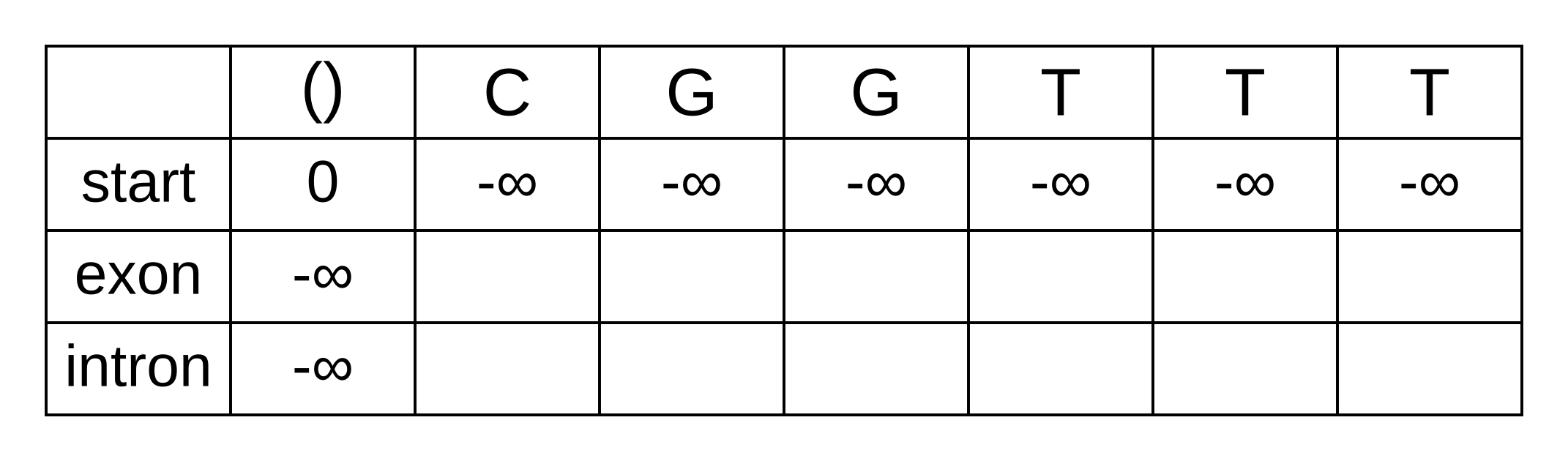
The transition log probability from any state to the start state is -∞, so for any value of i from 1 onwards, v_start,i = -∞. Go ahead and fill those in to save time:

For the next element v_exon,1 we only have to consider the transition from the start state to the exon state, because that is the only transition permitted by the model. Even if we do the calculations for the other transitions, the results of those calculations will be negative infinities because the Viterbi probability of non-start states in the first column are negative infinities. The log-probability at v_exon,1 is therefore:

• v_exon,1 = v_start,0 + t_start,exon + e_exon,1 = 0 + 0 + -1.61 = -1.61

The log-probability of v_intron,1 is negative infinity because the model does not permit the state at the first sequence position to be an intron. This can be effected computationally by setting the t_start,intron log-probability to negative infinity. Then regardless of the Viterbi and emission log-probabilities, the sum of v, t and e will be negative infinity.

Fill in both values for the first position of the sequence (or second column of the matrix), and add a pointer from the exon state to the start state:

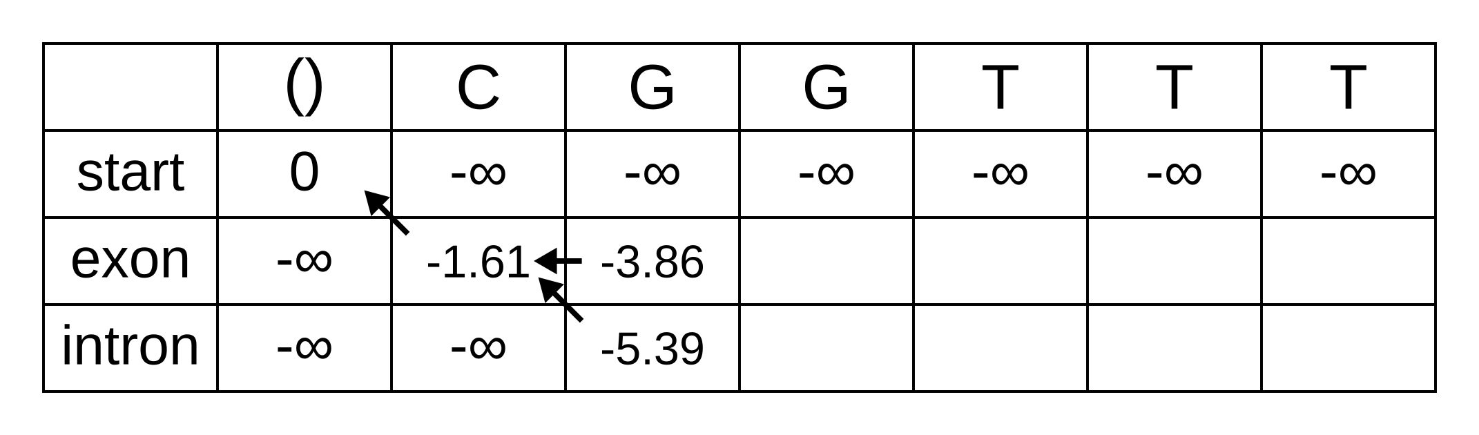
Once we get to v_exon,2, we only have to consider the exon to exon transition since the log-probabilities for the other states at the previous position are negative infinities. So this log-probability will be:

• v_exon,2 = v_exon,1 + t_exon,exon + e_exon,2 = -1.61 + -0.21 + -2.04 = -3.86

And for the same reason to calculate v_intron,2 we only have to consider the exon to intron transition, and this log-probability will be:

• v_intron,2 = v_exon,1 + t_exon,intron + e_intron,2 = -1.61 + -1.66 + -2.12 = -5.39

So fill on those values, and add pointers to the only permitted previous state, which is the exon state:

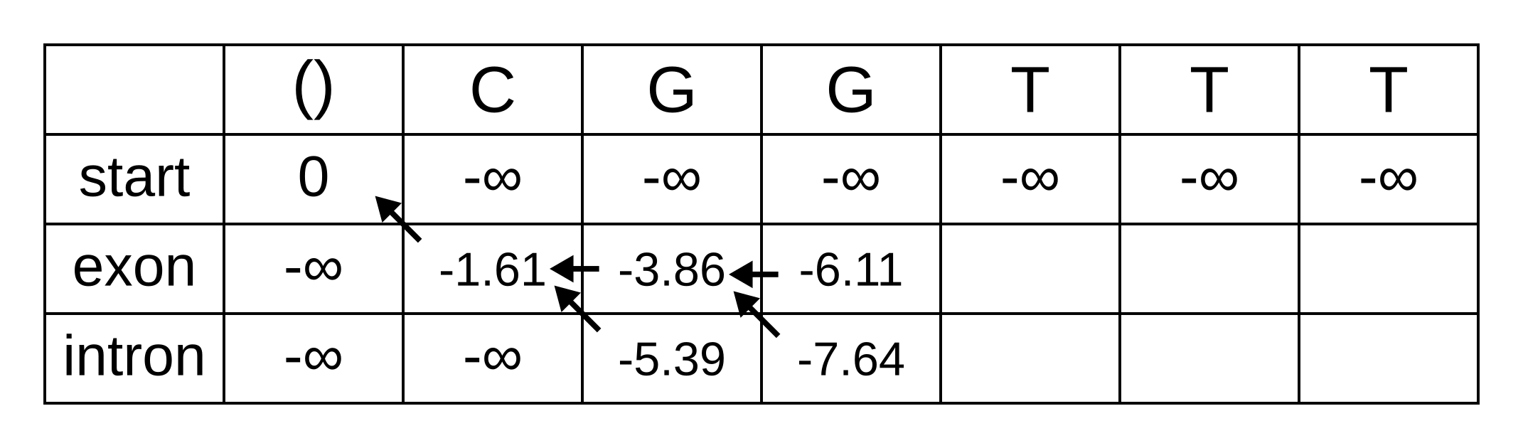
For the next position, we have to consider all transitions between intron or exon to intron or exon since both of those states have finite log-probabilities at the previous position. The log-probability of v_exon,3 will be the maximum of:

• v_exon,2 + t_exon,exon + e_exon,3 = -3.86 + -0.21 + -2.04 = -6.11
• v_intron,2 + t_intron,exon + e_exon,3 = -5.39 + -2.04 + -2.04 = -9.47

The previous hidden state that maximizes the Viterbi log-probability for the exon state at the third sequence position is therefore the exon state, and the maximum log-probability is -6.11. The log-probability of v_intron,3 will be the maximum of:

• v_exon,2 + t_exon,intron + e_intron,3 = -3.86 + -1.66 + -2.12 = -7.64
• v_intron,2 + t_{intron,intron} + e_intron,3 = -5.39 + -0.14 + -2.12 = -7.65

The previous hidden state that maximizes the Viterbi log-probability for the intron state at the third sequence position is therefore also the exon state, and the maximum log-probability is -7.64.

Fill in the maximum log-probabilities for each hidden state k, and also draw pointers to the previous hidden states corresponding to those maximum log-probabilities:

The rest of the matrix is filled in the same way as for the third position:

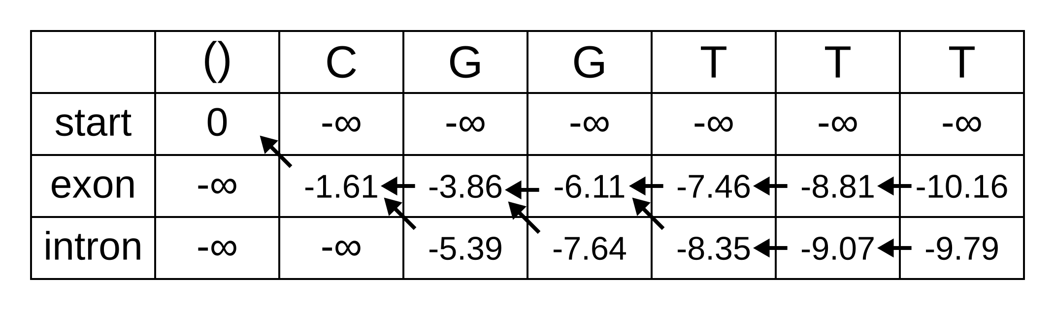
The maximum log joint probability of the sequence and path is the maximum out of v_k,L, where L is the length of the sequence. In other words, if we calculate the log joint probability

v_k,L = max_path1..L-1(logP(seq_0..L, path_0..L-1, path_L = k)).

for every value of k, we can identify the maximum log joint probability unconditional on the value of k at L. The path is then reconstructed by following the pointers backwards from the maximum log joint probability. In our toy example, the maximum log joint probability is -9.79 and the path is:

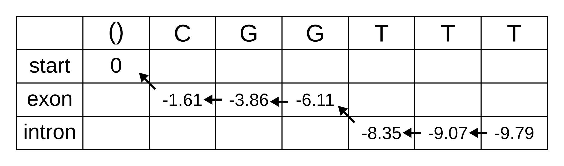
Or, ignoring the start state, exon-exon-exon-intron-intron-intron.

The basic Viterbi algorithm has a number of important properties:

• Its space and time complexity is O(Ln) and O(Ln²) respectively, where n is the number of states and L is the length of the sequence
• It returns a point estimate rather than a probability distribution
• Like Needleman–Wunsch or Smith–Waterman it is exact, so it is guaranteed to find the optimal¹ solution, unlike heuristic algorithms, and unlike an MCMC chain run for a finite number of steps²
• The probability is the (log) joint probability of the entire sequence (e.g. nucleotides or amino acids) and the entire path of unobserved states. It is not identifying the most probable hidden state at each position, because it is not marginalizing over the hidden states at other positions.

If the joint probability is close to sum of all joint probabilities, in other words if there are no other plausible state paths, then the point estimate returned by the algorithm will be reliable. Let’s see how it performs for our splice site model. The following code implements the Viterbi algorithm by reading in a previously inferred HMM to analyze a novel sequence:

import csv
import numpy
import sys

neginf = float("-inf")

def read_fasta(fasta_path):
	label = None
	sequence = None

	fasta_sequences = {}

	fasta_file = open(fasta_path)

	l = fasta_file.readline()
	while l != "":
		if l[0] == ">":
			if label != None:
				fasta_sequences[label] = sequence

			label = l[1:].strip()
			sequence = ""
		elif label != None:
			sequence += l.strip()

		l = fasta_file.readline()

	fasta_file.close()

	if label != None:
		fasta_sequences[label] = sequence

	return fasta_sequences

def read_matrix(matrix_path):
	matrix_file = open(matrix_path)
	matrix_reader = csv.reader(matrix_file)

	column_names = next(matrix_reader)

	list_of_numeric_rows = []
	for row in matrix_reader:
		numeric_row = numpy.array([float(x) for x in row])
		list_of_numeric_rows.append(numeric_row)

	matrix_file.close()

	matrix = numpy.stack(list_of_numeric_rows)

	return column_names, matrix

# ignore warnings caused by zero probability states
numpy.seterr(divide = "ignore")

emission_matrix_path     = sys.argv[1]
transmission_matrix_path = sys.argv[2]
fasta_path               = sys.argv[3]

sequence_alphabet, e_matrix = read_matrix(emission_matrix_path)
hidden_state_alphabet, t_matrix = read_matrix(transmission_matrix_path)

log_e_matrix = numpy.log(e_matrix)
log_t_matrix = numpy.log(t_matrix)

m = len(hidden_state_alphabet) # the number of hidden states

fasta_sequences = read_fasta(fasta_path)

for sequence_name in fasta_sequences:
	sequence = fasta_sequences[sequence_name]

	n = len(sequence) # the length of the sequence and index of the last position

	# the first character is also offset by 1, for pseudo-1-based-addressing
	numeric_sequence = numpy.zeros(n + 1, dtype = numpy.uint8)
	for i in range(n):
		numeric_sequence[i + 1] = sequence_alphabet.index(sequence[i])

	# all calculations will be in log space
	v_matrix = numpy.zeros((m, n + 1)) # Viterbi log probabilities
	p_matrix = numpy.zeros((m, n + 1), dtype = numpy.uint8) # Viterbi pointers

	# initialize matrix probabilities
	v_matrix.fill(neginf)
	v_matrix[0, 0] = 0.0

	temp_vitebri_probabilities = numpy.zeros(m)

	for i in range(1, n + 1):
		for k in range(1, m): # state at i
			for j in range(m): # state at i - 1
				e = log_e_matrix[k, numeric_sequence[i]]
				t = log_t_matrix[j, k]
				v = v_matrix[j, i - 1]

				temp_vitebri_probabilities[j] = e + t + v

			v_matrix[k, i] = numpy.max(temp_vitebri_probabilities)
			p_matrix[k, i] = numpy.argmax(temp_vitebri_probabilities)

	# initialize the maximum a posteriori hidden state path using the state with
	# the highest joint probability at the last position
	map_state = numpy.argmax(v_matrix[:, n])

	# then follow the pointers backwards from (n - 1) to 0
	for i in reversed(range(n)):
		subsequent_map_state = map_state
		map_state = p_matrix[subsequent_map_state, i + 1]

		if map_state != subsequent_map_state:
			print("Transition from %s at position %d to %s at position %d" % (hidden_state_alphabet[map_state], i, hidden_state_alphabet[subsequent_map_state], i + 1))

The first and second arguments for this program are paths to the emission matrix and transmission matrix respectively. A simplified version of the emission matrix from the previously inferred gene structure HMM looks like this:

A,C,G,T
0.0000,0.0000,0.0000,0.0000
0.2905,0.2018,0.2349,0.2728
0.0952,0.0327,0.7735,0.0986
0.0011,0.0000,0.9988,0.0001
0.2786,0.1581,0.1581,0.4052
0.0000,0.0010,0.9989,0.0001
0.2535,0.1039,0.5197,0.1229

And a simplified version of the transition matrix looks like this:

start,exon interior,exon 3',intron 5',intron interior,intron 3',exon 5'
0.0000,1.0000,0.0000,0.0000,0.0000,0.0000,0.0000
0.0000,0.9962,0.0038,0.0000,0.0000,0.0000,0.0000
0.0000,0.0000,0.0000,1.0000,0.0000,0.0000,0.0000
0.0000,0.0000,0.0000,0.0000,1.0000,0.0000,0.0000
0.0000,0.0000,0.0000,0.0000,0.9935,0.0065,0.0000
0.0000,0.0000,0.0000,0.0000,0.0000,0.0000,1.0000
0.0000,1.0000,0.0000,0.0000,0.0000,0.0000,0.0000

We can analyse the Arabidopsis gene FOLB2 (which codes for an enzyme that is part of the folate biosynthesis pathway). Warning: this is committing the cardinal sin of testing a model using data from the training set, which you should not do in real life! This gene has two introns, one within the 5’ untranslated region (UTR) and the other inside the coding sequence.

The third argument of the program is a path to a FASTA format sequence file, and the sequence of FOLB2 between the UTRs in FASTA format is:

>FOLB2
ATGGAGAAAGACATGGCAATGATGGGAGACAAACTGATACTGAGAGGCTTGAAATTTTATGGTTTCCATGGAGCTATTCC
TGAAGAGAAGACGCTTGGCCAGATGTTTATGCTTGACATCGATGCTTGGATGTGTCTCAAAAAGGCTGGTCTATCAGACA
ACTTAGCTGATTCTGTCAGCTATGTCGACATTTACAAGTTAGTTTTAATTACTAATATGAGAGGATTTGCTAGAGATAGT
TAACTAAATTCTCCCCTTTACTCTTGACCAATCCATTTTTATTGTGACCTCATCCAAAAATGACAAGCTTTGCTTATATA
ACAATTTGTCATCACTATCTGTGTCACTGAGTGATGCATTGATTATAGGATATGAAATGATTCTTTGAGATTGAAGATTT
GAAAAGGTTGTGTGTAGGTTATGTAGTAGTGACTACACTTTTCATATGCTGTGTTTGAAACTGTATCATAATTTGTTTTG
GAATGGAATGAATAATCTTAGCGTGGCAAAGGAAGTTGTAGAAGGGTCATCAAGAAACCTTCTGGAGAGAGTTGCAGGAC
TTATAGCTTCCAAAACTCTGGAAATATCCCCTCGGATAACAGCTGTTCGAGTGAAGCTATGGAAGCCAAATGTTGCGCTT
ATTCAAAGCACTATCGATTATTTAGGTGTCGAGATTTTCAGAGATCGCGCAACTGAATAA

Save the matrices and sequences to their own files, then run the Viterbi code with the paths to those files as the arguments. The Viterbi algorithm does detect an intron, but it gets the splice site positions wrong. This failure demonstrates the core problem of the algorithm on its own; it gives us an answer but without any sense of its probability. For that, we need the forward and backward algorithms.

For another perspective on the Viterbi algorithm, consult lesson 10.6 of Bioinformatics Algorithms by Compeau and Pevzner.

1. Optimal in the sense of finding the true maximum a posteriori (MAP) solution, not in the sense of finding the true path. ↩

2. MCMC run for an infinite number of steps should also be exact (conditional on the Markov chain being ergodic). In practice, because we do not have infinite time to conduct scientific research, MCMC is not guaranteed to sample exactly proportionally to the target distribution. ↩