
UPGMA and WPGMA trees
Two related methods for infer phylogenetic trees from multiple sequence alignments (MSAs) are the Unweighted Pair Group Method with Arithmetic Mean (UPMGA) and the Weighted Pair Group Method with Arithmetic Mean (WPGMA). Both are bottom-up clustering methods which work by connecting similar sequences first, then more distant sequences.
UPGMA and WPGMA infer ultrametric trees. These are trees which can be plotted as following a time axis and where the tips line up at time t = 0. The time axis of UPGMA and WPGMA inferred trees is in substitutions per site.
If a multiple sequence alignment is generated by the evolution of an ancestral sequence at the root node along the tree to the tips at a constant substitution (or mutation) rate, the sequence is said to be “clock-like”. When the substitution rate of the sequence is known, the genetic distances can be converted into times. In other words, the sequences in the present can be used as a clock to estimate the exact timing of nodes in the past!
Consider the left hand side tree, where the time axis (y-axis) is in substitutions per site: Let’s say that the substitution rate is 0.01 substitutions per site per million years. Then we can rescale the y-axis by this rate to derive the right hand side tree which is millions of years:
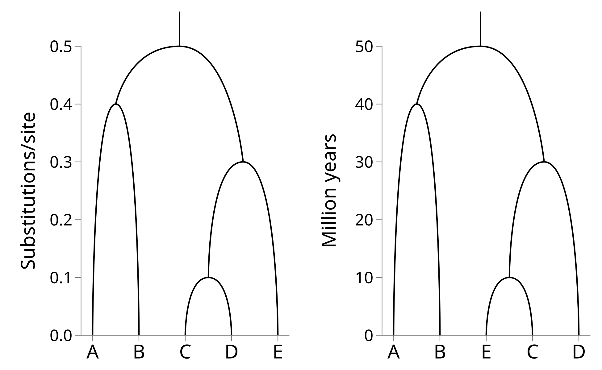
Because the inferred trees are ultrametric, UPGMA and WPGMA are implicitly assuming the sequence data is generated by a molecular clock. If the molecular clock is violated these methods should not be used.
Now we will learn how to simulate sequences from the above example tree, and use the simulated MSA to reconstruct the original tree using UPGMA. Our example tree can be encoded using the following Newick string:
((A:0.3,B:0.3):0.1,((C:0.1,D:0.1):0.1,E:0.2):0.2);
If we save this string as a file named “example.tree”, we can use the nucleotide and amino acid sequence simulation tool Seq-Gen to generate the MSA. The following command will sample a nucleotide sequence of 30 characters in length, evolve it under the Jukes–Cantor model to create an MSA, and save it to a new file with the name “example.phy”:
seq-gen -mHKY -l30 -op example.tree > example.phy
The example MSA generated by the above command follows:
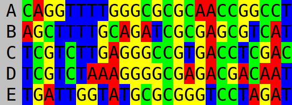
The first step when reconstructing a tree using UPGMA (or WPGMA) is to calculate a distance matrix from the sequence data. We will apply the Jukes–Cantor model again here, which makes calculating the distance matrix trivial. First count the number of sites which differ between each pair of sequences in the MSA:
| A | B | C | D | E | |
|---|---|---|---|---|---|
| A | 0 | 13 | 15 | 15 | 15 |
| B | 13 | 0 | 14 | 16 | 15 |
| C | 15 | 14 | 0 | 8 | 13 |
| D | 15 | 16 | 8 | 0 | 14 |
| E | 15 | 15 | 13 | 14 | 0 |
From this, calculate the P-distance between each sequence pair. This is simply the proportion of sites which differ, or the elements above divided by the sequence length, which in this case is 25:
| A | B | C | D | E | |
|---|---|---|---|---|---|
| A | 0.00 | 0.52 | 0.60 | 0.60 | 0.60 |
| B | 0.52 | 0.00 | 0.56 | 0.64 | 0.60 |
| C | 0.60 | 0.56 | 0.00 | 0.32 | 0.52 |
| D | 0.60 | 0.64 | 0.32 | 0.00 | 0.56 |
| E | 0.60 | 0.60 | 0.52 | 0.56 | 0.00 |
Under the Jukes–Cantor model, the genetic distance is simply -(3/4) × log(1 - (4/3) × p), where p is the P-distance:
| A | B | C | D | E | |
|---|---|---|---|---|---|
| A | 0.00 | 0.89 | 1.21 | 1.21 | 1.21 |
| B | 0.89 | 0.00 | 1.03 | 1.44 | 1.21 |
| C | 1.21 | 1.03 | 0.00 | 0.42 | 0.89 |
| D | 1.21 | 1.44 | 0.42 | 0.00 | 1.03 |
| E | 1.21 | 1.21 | 0.89 | 1.03 | 0.00 |
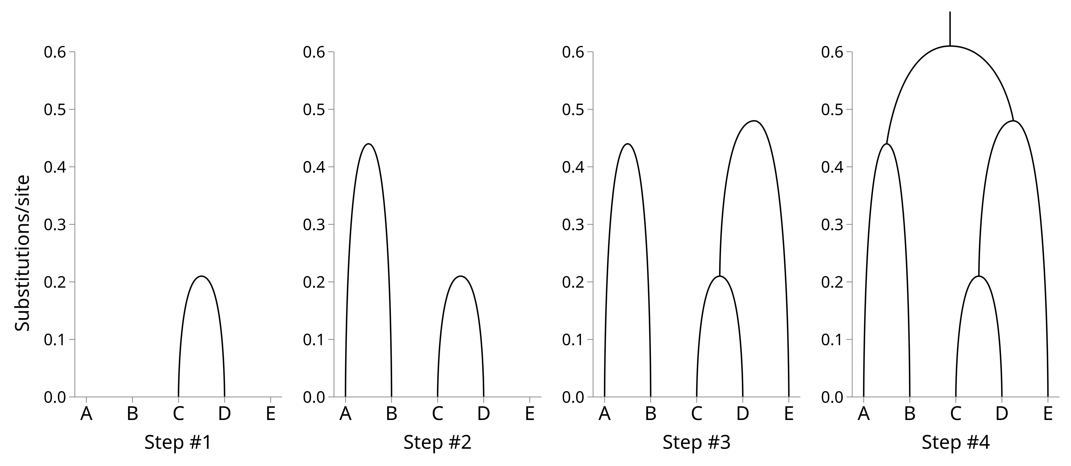
Now we can build the tree by shrinking the distance matrix by one row and column at a time. First identify the off-diagonal element of the distance matrix with the lower value. In this case it is row C by column D (or vice versa as the matrix is symmetric), with a value of 0.42. Use half this value as the height of a node which merges C and D.
Merge the two rows and the two columns. We can designate this node by the number 5, leaving numbers 0 through 4 free for the leaf nodes. For each element in the new row, calculate its value as the average of the original distances, weighted by the number of taxa below the corresponding nodes. For example, when calculating the distance from 5 to B, the original distances are 1.03 (C to B) and 1.44 (D to B). There is one taxon (C) below the corresponding node for row C, and one taxon (D) below the corresponding node for D.
The new distance is therefore (1.03 × 1 / 2) + (1.44 × 1 / 2) = 1.23. Filling the rest of the new row and column in:
| A | B | 5 | E | |
|---|---|---|---|---|
| A | 0.00 | 0.89 | 1.21 | 1.21 |
| B | 0.89 | 0.00 | 1.23 | 1.21 |
| 5 | 1.21 | 1.23 | 0.00 | 0.96 |
| E | 1.21 | 1.21 | 0.96 | 0.00 |
The lowest off-diagonal value is now 0.89, so we will merge A and B. The height of the A–B node will be 0.5 × 0.89 = 0.44. Merge the A and B rows and columns using their weighted averages, like before:
| 6 | 5 | E | |
|---|---|---|---|
| 6 | 0.00 | 1.22 | 1.21 |
| 5 | 1.22 | 0.00 | 0.96 |
| E | 1.21 | 0.96 | 0.00 |
The lowest off-diagonal value is now 0.96, so we will merge E and the internal node 5. The new node height will be 0.48. Calculating the new distance matrix nicely demonstrates how weighting is used. There is one taxon (E) below the corresponding node for row E, and two taxa (C and D) below the corresponding node for row 5. The distance from 6 to 7 will be the average of the original distances weighted by their taxon counts = (1.21 × 1 / 3) + (1.22 × 2 / 3) = 1.22.
| 6 | 7 | |
|---|---|---|
| 6 | 0.00 | 1.22 |
| 7 | 1.22 | 0.00 |
The root node height will therefore be 1.22 × 0.5 = 0.61. You can see how the tree is constructed from the bottom up:
WPGMA is the same as UPGMA, except when shrinking the distance matrices, the new row and column values are no longer weighted by the number of taxa. Yes that’s right, Unweighted PGMA is based on weighted averages, and Weighted PGMA is based on unweighted averages. Good luck remembering this confusing difference!